Question

Solve the following differential equation using MATLAB's ODE45 function. Assume that the all initial conditions are zero and that the input to the system, /(t), is a unit step The output of interest is x dt dt dt To make use of the ODE45 function for this problem, the equation should be expressed in state variable form as shown below Solve the original differential equation for the highest derivative dt 2 dt Assign the following state variables dt dt Express the original differential equation in state variable form dr 71 2 dtdt 2 2 2-1-2-2-2-3 +_f(t) dt dt 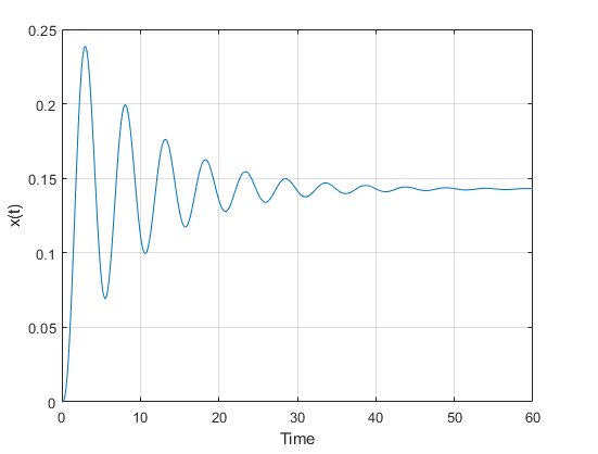Or, in matrix form as: -5/2-2-7/2Tal 「1/2 0 Recall that the syntax for the ODE45 function call is: [TOUT,YOUT] = ODE45('ODEFUN,TSPAN,Y0) Let the time span, TSPAN = [060]. Set all initial conditions (Y0) to zero. Plot x(t) from 0 to 60 seconds. Label the vertical axis x(t)' and the horizontal axis Time". Turn on the grid for this plot. Copy the following to your solution document: The script file that you created to call ODE45 and for plotting the results. The function that you created (named ODEFUN above) to calculate the state variable derivatives. The figure you created. Use the Copy Figure' option under the figure Edit menu and then paste your result into your solution document. NOTE: Your use of ODE45 will generate the time response of all three state variables. You are to plot x(t) which is the third state variable. Your plot command will be something like plot (t,z(:,3))

Answer 1

%。defun is at bottom, you can also define separate function file for that tspan = [0 60]; % lime span 20- [O Ο Ο]; % Initial conditions [z1 (0) z2 (0) z3 (0)] (all zero) plot (t, z(:,3)) xlabel ("Time" ylabel ("x(t)") grid on function z dot = odefun (t,2) % Unit Step function mati -5/2 -2 -7/2: 1 0 0:. 0 1 01: mat2 = [1/2 :0; 01: z-dot mat1*[2 (1):2 (2):2(3)] + mat2+f(t); State-variable matrix form - end

0.25 0.2 0.15 0.1 0.05 10 20 30 Time 40 50 60

Text :-

tspan = [0 60]; % Time span
z0 = [0 0 0];   % Initial conditions [z1(0) z2(0) z3(0)] (all zero)

[t,z] = ode45(@(t,z)odefun(t,z), tspan, z0);

plot(t,z(:,3))
xlabel("Time")
ylabel("x(t)")
grid on

function z_dot = odefun(t,z)
    f = @(t) 1;         % Unit Step function
    mat1 = [-5/2 -2 -7/2;...
              1   0   0;...
              0   1   0];
    mat2 = [1/2 ;0; 0];

    z_dot = mat1*[z(1);z(2);z(3)] + mat2*f(t);  % State-Variable matrix form
end