
Homework Answers
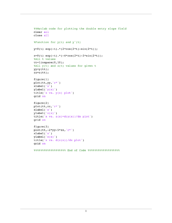
%%Matlab code for plotting the double entry slope field
clear all
close all
%Function for y(t) and y'(t)
y=@(t) exp(-t).*(2*cos(2*t)-sin(2*t));
z=@(t) exp(-t).*(-4*cos(2*t)-3*sin(2*t));
%All t values
tt=linspace(0,10);
%All y(t) and z(t) values for given t
yy=y(tt);
zz=z(tt);
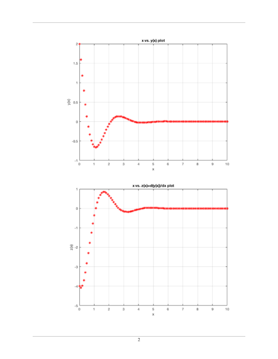
figure(1)
plot(tt,yy,'r*')
xlabel('x')
ylabel('y(x)')
title('x vs. y(x) plot')
grid on
figure(2)
plot(tt,zz,'r*')
xlabel('x')
ylabel('z(x)')
title('x vs. z(x)=d(y(x))/dx plot')
grid on
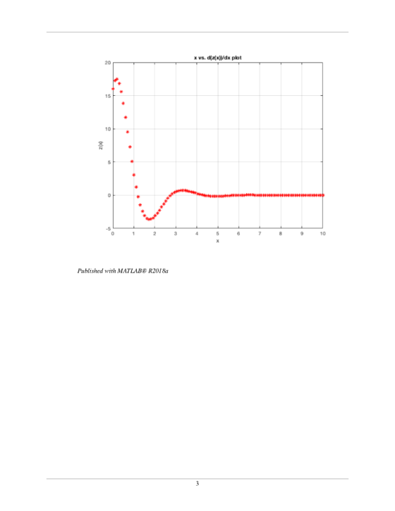
figure(3)
plot(tt,-2*yy-5*zz,'r*')
xlabel('x')
ylabel('z(x)')
title('x vs. d(z(x))/dx plot')
grid on
%%%%%%%%%%%%%%%%%%% End of Code %%%%%%%%%%%%%%%%%%%
Add Answer to:
A second order differential equation can be graphed by using a double entry slopefield (lety,so '...
A second order differential equation can be graphed by using a double entry slopefield (lety,so '...
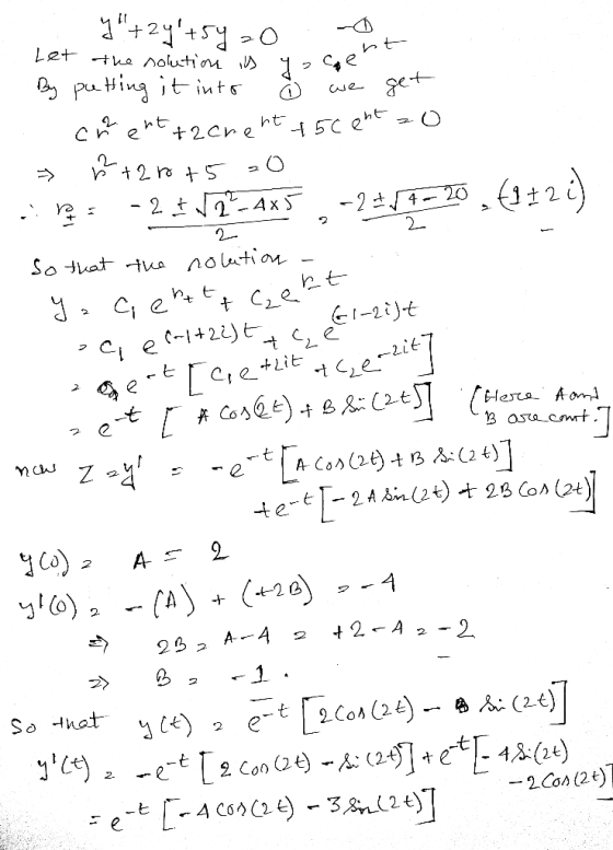
 A second order differential equation can be graphed by using a double entry slopefield (lety,so '. Find the exact solution to the second-order differential equation y"+2y+5y 0 with initial conditions y(o)-2 and y (o--4, then graph with the double entry slopefield plot below. (5pts) RAD Examl 1.1 0.2 Exanill (04 0 2 -2 .2
A second order differential equation can be graphed by using a double entry slopefield (lety,so '. Find the exact solution to the second-order differential equation y"+2y+5y...
A second order differential equation can be graphed by using a double entry slopefield (lety,so '. Find the exact solution to the second-order differential equation y"+2y+5y 0 with initial conditions y(o)-2 and y (o--4, then graph with the double entry slopefield plot below. (5pts) RAD Examl 1.1 0.2 Exanill (04 0 2 -2 .2
A second order differential equation can be graphed by using a double entry slopefield (lety,so '. Find the exact solution to the second-order differential equation y"+2y+5y...
answer in matlab code Employ the bvp4c command to find the approximate solution of the boundary value problem governed by the second-order nonhomogeneous differential equation, 9. with the bound...
 answer in matlab code
Employ the bvp4c command to find the approximate solution of the boundary value problem governed by the second-order nonhomogeneous differential equation, 9. with the boundary conditions of y(0) 5 and y(1)-2. Plot to compare the approximate solution with the exact solution obtained by using the dsolve command.
Employ the bvp4c command to find the approximate solution of the boundary value problem governed by the second-order nonhomogeneous differential equation, 9. with the boundary conditions of y(0) 5...
answer in matlab code
Employ the bvp4c command to find the approximate solution of the boundary value problem governed by the second-order nonhomogeneous differential equation, 9. with the boundary conditions of y(0) 5 and y(1)-2. Plot to compare the approximate solution with the exact solution obtained by using the dsolve command.
Employ the bvp4c command to find the approximate solution of the boundary value problem governed by the second-order nonhomogeneous differential equation, 9. with the boundary conditions of y(0) 5...
1- Use the Reduction of Order method to find a second solution of the equation 4x2y"...
 1- Use the Reduction of Order method to find a second solution of the equation 4x2y" + y = 0 Given that yı = xì Inx 2- Solve the differential equation y" + 4y + 4y = 0 3- Solve the differential equation y" + 2y + 10y = 0 y” + 5y + 4y = cosx + 2e*
please write the code for the plot Solve the following second order differential equation analytically for...
 please write the code for the plot
Solve the following second order differential equation analytically for x(t): - dx + 5x = 8 * 2 for the following two cases: Case 1: all initial conditions are zero. Case 2: given the initial conditions: x (0) = 1 (0) = 2 For both cases, also plot the solution obtained, for t = 0 to 10.
please write the code for the plot
Solve the following second order differential equation analytically for x(t): - dx + 5x = 8 * 2 for the following two cases: Case 1: all initial conditions are zero. Case 2: given the initial conditions: x (0) = 1 (0) = 2 For both cases, also plot the solution obtained, for t = 0 to 10.
Please assist with the following using Laplace Transform The second order differential equation of a vibratıng...
 Please assist with the following using Laplace
Transform
The second order differential equation of a vibratıng system is given by d2 dt'dt 5 1 Determine the system transfer function with initial conditions y(0) y(0)0 5 2 Determine the response of the system, y(t), with a unit step input r(t) and intial conditions y(0)1 and y(0) -1 (15)
Please assist with the following using Laplace
Transform
The second order differential equation of a vibratıng system is given by d2 dt'dt 5 1 Determine the system transfer function with initial conditions y(0) y(0)0 5 2 Determine the response of the system, y(t), with a unit step input r(t) and intial conditions y(0)1 and y(0) -1 (15)
Solve the second order differential equation for an LRC circuit in series with the initial conditions...
 Solve the second order differential equation for an LRC circuit in
series with the initial conditions given. And create a graph
(100x10->) + (470) ** (470x10-69 Con las condiciones iniciales siguientes: g(0)=0 y (0)=0.
Solve the second order differential equation for an LRC circuit in
series with the initial conditions given. And create a graph
(100x10->) + (470) ** (470x10-69 Con las condiciones iniciales siguientes: g(0)=0 y (0)=0.
Problem 4. The higher order differential equation and initial conditions are shown as follows: = dy...
 Problem 4. The higher order differential equation and initial conditions are shown as follows: = dy dy +y?, y(0) = 1, y'(0) = -1, "(0) = 2 dt3 dt (a) [5pts. Transform the above initial value problem into an equivalent first order differential system, including initial conditions. (b) [2pts.] Express the system and the initial condition in (a) in vector form. (c) [4pts.] Using the second order Runge Kutta method as follows Ū* = Ūi + hĚ(ti, Ūi) h =...
The graphs of a member of a family of solutions of a second order differential equation...
 The graphs of a member of a family of solutions of a second order differential equation given. Match the solutions curve with a pair of initial conditions. 2-1(2, 4 v) 1. D 2. B y(0) = 2, y'(0) = -2 4 -2 y(0) = 1, y'(0) = 1/2 y(0) = 2, y'(0) = 0 3. с
A system of two first order differential equations can be written as: A second order explicit R...
A system of two first order differential equations can be written as: A second order explicit Runge-Kutta scheme for the system of two first order equations is Consider the following second order differential equation: Use the Runge-kutta scheme to find an approximate solution of the second order differential equation, at x = 0.2, if the step size h = 0.1. Maintain at least eight decimal digit accuracy throughout all your calculations. You may express your answer as a five decimal...
(1) Solve the differential equation y 2xy, y(1)= 1 analytically. Plot the solution curve for the interval x 1 to 2 (see...
 (1) Solve the differential equation y 2xy, y(1)= 1 analytically. Plot the solution curve for the interval x 1 to 2 (see both MS word and Excel templates). 3 pts (2) On the same graph, plot the solution curve for the differential equation using Euler's method. 5pts (3) On the same graph, plot the solution curve for the differential equation using improved Euler's method. 5pts (4) On the same graph, plot the solution curve for the differential equation using Runge-Kutta...
 A second order differential equation can be graphed by using a double entry slopefield (lety,so '. Find the exact solution to the second-order differential equation y"+2y+5y 0 with initial conditions y(o)-2 and y (o--4, then graph with the double entry slopefield plot below. (5pts) RAD Examl 1.1 0.2 Exanill (04 0 2 -2 .2
A second order differential equation can be graphed by using a double entry slopefield (lety,so '. Find the exact solution to the second-order differential equation y"+2y+5y...
A second order differential equation can be graphed by using a double entry slopefield (lety,so '. Find the exact solution to the second-order differential equation y"+2y+5y 0 with initial conditions y(o)-2 and y (o--4, then graph with the double entry slopefield plot below. (5pts) RAD Examl 1.1 0.2 Exanill (04 0 2 -2 .2
A second order differential equation can be graphed by using a double entry slopefield (lety,so '. Find the exact solution to the second-order differential equation y"+2y+5y...
 answer in matlab code
Employ the bvp4c command to find the approximate solution of the boundary value problem governed by the second-order nonhomogeneous differential equation, 9. with the boundary conditions of y(0) 5 and y(1)-2. Plot to compare the approximate solution with the exact solution obtained by using the dsolve command.
Employ the bvp4c command to find the approximate solution of the boundary value problem governed by the second-order nonhomogeneous differential equation, 9. with the boundary conditions of y(0) 5...
answer in matlab code
Employ the bvp4c command to find the approximate solution of the boundary value problem governed by the second-order nonhomogeneous differential equation, 9. with the boundary conditions of y(0) 5 and y(1)-2. Plot to compare the approximate solution with the exact solution obtained by using the dsolve command.
Employ the bvp4c command to find the approximate solution of the boundary value problem governed by the second-order nonhomogeneous differential equation, 9. with the boundary conditions of y(0) 5...
 1- Use the Reduction of Order method to find a second solution of the equation 4x2y" + y = 0 Given that yı = xì Inx 2- Solve the differential equation y" + 4y + 4y = 0 3- Solve the differential equation y" + 2y + 10y = 0 y” + 5y + 4y = cosx + 2e*
 please write the code for the plot
Solve the following second order differential equation analytically for x(t): - dx + 5x = 8 * 2 for the following two cases: Case 1: all initial conditions are zero. Case 2: given the initial conditions: x (0) = 1 (0) = 2 For both cases, also plot the solution obtained, for t = 0 to 10.
please write the code for the plot
Solve the following second order differential equation analytically for x(t): - dx + 5x = 8 * 2 for the following two cases: Case 1: all initial conditions are zero. Case 2: given the initial conditions: x (0) = 1 (0) = 2 For both cases, also plot the solution obtained, for t = 0 to 10.
 Please assist with the following using Laplace
Transform
The second order differential equation of a vibratıng system is given by d2 dt'dt 5 1 Determine the system transfer function with initial conditions y(0) y(0)0 5 2 Determine the response of the system, y(t), with a unit step input r(t) and intial conditions y(0)1 and y(0) -1 (15)
Please assist with the following using Laplace
Transform
The second order differential equation of a vibratıng system is given by d2 dt'dt 5 1 Determine the system transfer function with initial conditions y(0) y(0)0 5 2 Determine the response of the system, y(t), with a unit step input r(t) and intial conditions y(0)1 and y(0) -1 (15)
 Solve the second order differential equation for an LRC circuit in
series with the initial conditions given. And create a graph
(100x10->) + (470) ** (470x10-69 Con las condiciones iniciales siguientes: g(0)=0 y (0)=0.
Solve the second order differential equation for an LRC circuit in
series with the initial conditions given. And create a graph
(100x10->) + (470) ** (470x10-69 Con las condiciones iniciales siguientes: g(0)=0 y (0)=0.
 Problem 4. The higher order differential equation and initial conditions are shown as follows: = dy dy +y?, y(0) = 1, y'(0) = -1, "(0) = 2 dt3 dt (a) [5pts. Transform the above initial value problem into an equivalent first order differential system, including initial conditions. (b) [2pts.] Express the system and the initial condition in (a) in vector form. (c) [4pts.] Using the second order Runge Kutta method as follows Ū* = Ūi + hĚ(ti, Ūi) h =...
 The graphs of a member of a family of solutions of a second order differential equation given. Match the solutions curve with a pair of initial conditions. 2-1(2, 4 v) 1. D 2. B y(0) = 2, y'(0) = -2 4 -2 y(0) = 1, y'(0) = 1/2 y(0) = 2, y'(0) = 0 3. с
 (1) Solve the differential equation y 2xy, y(1)= 1 analytically. Plot the solution curve for the interval x 1 to 2 (see both MS word and Excel templates). 3 pts (2) On the same graph, plot the solution curve for the differential equation using Euler's method. 5pts (3) On the same graph, plot the solution curve for the differential equation using improved Euler's method. 5pts (4) On the same graph, plot the solution curve for the differential equation using Runge-Kutta...
Most questions answered within 3 hours.
-
What would you expect the observed boiling point to be at 10
torrs of a liquid...
asked 2 minutes ago -
write a javascript jquery code to display calendar and let it be
sticked on the textbox...
asked 10 minutes ago -
A Call Spread is
A.
The simultaneous purchase of a call and
sale of a put...
asked 9 minutes ago -
In response to concerns about a future recession, the government
decides to give consumers a tax...
asked 11 minutes ago -
Experimental studies of cancer often use strains of animals that
have a naturally high incidence of...
asked 17 minutes ago -
Sociology Question Emile Durkheim
What role does mass media play in the lives of contemporary
citizens?...
asked 21 minutes ago -
Why would you silence gene expression for both wild-type and
mutants? I am on a question...
asked 30 minutes ago -
While all of the elements below are helpful, Booth et al. (2008)
emphasize that it is...
asked 35 minutes ago -
2. Use the three-step method to analyze the effects of the event
on the equilibrium price...
asked 35 minutes ago -
Draw a Venn diagram of three domains of life and explain.
asked 39 minutes ago -
In testing a new drug, researchers found that 5% of all patients
using it will have...
asked 1 hour ago -
List the six general types of information management systems,
and give one logistics application to each...
asked 59 minutes ago