
Here is the information that is needed for this work:
1 2 5 5 20 1 R2-29522 5 2 4 3 5 8 1 0 9 2 3 4 5 3 5 3 9 4 5 2 8 4 4 3 8 6 3 3 5 9 3 4 6 0 5 0 4 1027251 1 1 2 112 14456694518974191469644566466957464465944956794ー4 1 1 5 5 52 8 1 2 5 17 4 7 1 4 1 4 5 5 0 9 7 8 0 4 7 5 5 0 0 6 6 3 0 4 3 7 5 6 9 6 8 5 8 3 7 6 4 5 7 5 0 1573653634 2122 32122212221221 2112211112
Homework Answers
regression summary , coefficient table and F-test
| SUMMARY OUTPUT | |||||
| Regression Statistics | |||||
| Multiple R | 0.585123024 | ||||
| R Square | 0.342368953 | ||||
| Adjusted R Square | 0.299479971 | ||||
| Standard Error | 5.412552887 | ||||
| Observations | 50 | ||||
| ANOVA | |||||
| df | SS | MS | F | Significance F | |
| Regression | 3 | 701.5751592 | 233.8583864 | 7.982678579 | 0.00021757 |
| Residual | 46 | 1347.603523 | 29.29572876 | ||
| Total | 49 | 2049.178682 | |||
| Coefficients | Standard Error | t Stat | P-value | Lower 95% | |
| Intercept | 7.872986591 | 4.087193427 | 1.926257401 | 0.06026464 | -0.354107071 |
| EDUC | 1.437060506 | 0.338639743 | 4.243626263 | 0.000105402 | 0.755414058 |
| EXPER | 0.448282229 | 0.141867317 | 3.159869648 | 0.002789784 | 0.162718131 |
| AGE | -0.011386246 | 0.083422321 | -0.1364892 | 0.89203017 | -0.179306669 |
wage^ = 7.873 + 1.4371 Educ + 0.4483 Exper -0.0114 Age
yes, all signs are as expected
wage is positively correlated with Education and experience
and is negatively correlated with age
coefficient of Education is 1.4371
as education increases by 1 unit, on average wage will increase by
1.45 units
coefficient of detemrination = 0.3427
hence 34.27% of variation in wage is explained by this model
Add Answer to:
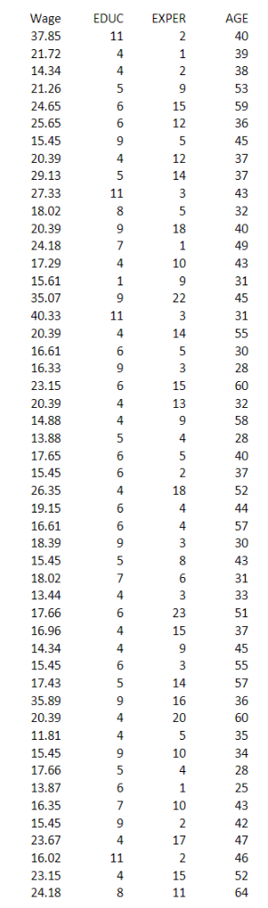
Here is the information that is needed for this work: A researcher interviews 50 employees of a large manufacturer and colects data on each worker's hourly wage (Wage), years of higher education...
A researcher interviews 50 employees of a large manufacturer and collects data on each worker’s h...
 A researcher interviews 50 employees of a large manufacturer and
collects data on each worker’s hourly wage (Wage), years of higher
education (EDUC), experience (EXPER), and age (AGE).
Wage
EDUC
EXPER
AGE
Male
37.85
11
2
40
1
21.72
4
1
39
0
⋮
⋮
⋮
⋮
⋮
24.18
8
11
64
0
A researcher interviews 50 employees of a large manufacturer and collects data on each worker's hourly wage (Wage), years of higher education (EDUC), experience (EXPER), and age...
A researcher interviews 50 employees of a large manufacturer and
collects data on each worker’s hourly wage (Wage), years of higher
education (EDUC), experience (EXPER), and age (AGE).
Wage
EDUC
EXPER
AGE
Male
37.85
11
2
40
1
21.72
4
1
39
0
⋮
⋮
⋮
⋮
⋮
24.18
8
11
64
0
A researcher interviews 50 employees of a large manufacturer and collects data on each worker's hourly wage (Wage), years of higher education (EDUC), experience (EXPER), and age...
Using data from 50 workers, a researcher estimates Wage = β0 + β1Education + β2Experience +...
Using data from 50 workers, a researcher estimates Wage = β0 + β1Education + β2Experience + β3Age + ε, where Wage is the hourly wage rate and Education, Experience, and Age are the years of higher education, the years of experience, and the age of the worker, respectively. The regression results are shown in the following table. Coefficients Standard Error t Stat p-Value Intercept 7.17 4.26 1.68 0.0991 Education 1.81 0.35 5.17 0.0000 Experience 0.45 0.10 4.50 0.0000 Age −0.01...
Using data from 50 workers, a researcher estimates Wage = β0 + β1Education + β2Experience +...
Using data from 50 workers, a researcher estimates Wage = β0 + β1Education + β2Experience + β3Age + ε, where Wage is the hourly wage rate and Education, Experience, and Age are the years of higher education, the years of experience, and the age of the worker, respectively. The regression results are shown in the following table. Coefficients Standard Error t Stat p-Value Intercept 7.73 3.94 1.96 0.0558 Education 1.15 0.39 2.95 0.0050 Experience 0.45 0.11 4.09 0.0002 Age −0.03...
Using data from 50 workers, a researcher estimates Wage = β0 + β1Education + β2Experience +...
Using data from 50 workers, a researcher estimates Wage = β0 + β1Education + β2Experience + β3Age + ε, where Wage is the hourly wage rate and Education, Experience, and Age are the years of higher education, the years of experience, and the age of the worker, respectively. The regression results are shown in the following table. Coefficients Standard Error t Stat p-Value Intercept 8.23 4.40 1.87 0.0678 Education 1.23 0.38 3.24 0.0022 Experience 0.53 0.18 2.94 0.0051 Age −0.08...
2 Using data from 50 workers, a researcher estimates Wage BoIEducation + 2Experience B3Age E, where...
 2 Using data from 50 workers, a researcher estimates Wage BoIEducation + 2Experience B3Age E, where Wage is the hourly wage rate and Education, Experience, and Age are the years of higher education, the years of experience, and the age of the worker respectively. The regression results are shown in the following table. 10 points Standard Coefficients t Stat P-Value 0.1310 0.0003 0.0022 Error 4.24 Intercept Education Experience Age 6.52 1.32 1.54 0.34 0.12 3.88 3.25 -0.20 0.39 0.01 0.05...
Using data from 50 workers, a researcher estimates Wage = ?0 + ?1Education + ?2Experience +...
Using data from 50 workers, a researcher estimates Wage = ?0 + ?1Education + ?2Experience + ?3Age + ?, where Wage is the hourly wage rate and Education, Experience, and Age are the years of higher education, the years of experience, and the age of the worker, respectively. The regression results are shown in the following table. Coefficients Standard Error t Stat p-Value Intercept 7.58 4.42 1.71 0.0931 Education 1.68 0.37 4.54 0.0000 Experience 0.35 0.18 1.94 0.0580 Age ?0.06...
>|10|1|00001100-10110100 )13-175576 3 3 5 3 4 5 53 548532762 332244445 35931-12 10-4-0 5 2 2 1 7 ...
 please answer this question subject about Business Statistics
thanks
>|10|1|00001100-10110100 )13-175576 3 3 5 3 4 5 53 548532762 332244445 35931-12 10-4-0 5 2 2 1 7 4 6 4 4 6 5 9 4 4 9 5 6 794 453991567557258 04693|44838468346011 |00 | 3 7 6 4 5 7 5 0 1 5 7 3 6 5 3 6 34 a 1001110011011000-1 10-01-0101| 0 0 10 2880724703 3524354534 09| 8 3 9 6 5 7 7 3 2093151508 43355343343444343532...
please answer this question subject about Business Statistics
thanks
>|10|1|00001100-10110100 )13-175576 3 3 5 3 4 5 53 548532762 332244445 35931-12 10-4-0 5 2 2 1 7 4 6 4 4 6 5 9 4 4 9 5 6 794 453991567557258 04693|44838468346011 |00 | 3 7 6 4 5 7 5 0 1 5 7 3 6 5 3 6 34 a 1001110011011000-1 10-01-0101| 0 0 10 2880724703 3524354534 09| 8 3 9 6 5 7 7 3 2093151508 43355343343444343532...
2. The following data were collected last semester on ten students. Complete a multiple regression analysis in which you use AGE (A), MATH PROFICIENCY (MP) (on a 1 –10 scale), and GENDER (G) (0 = male...
2. The following data were collected last semester on ten students. Complete a multiple regression analysis in which you use AGE (A), MATH PROFICIENCY (MP) (on a 1 –10 scale), and GENDER (G) (0 = male, 1 = female) as predictors of FINAL EXAM (FE) performance. Do this analysis in SPSS and then answer the following questions. Subject # A MP G FE 1 35 8 1 90 2 31 6 0 88 3 26 5 1 84 4 33...
1. Use Minitab to get the same type of output (including graphs) with the following Income/Education data as the li...
 1. Use Minitab to get the same type of output (including graphs) with the following Income/Education data as the little data set discussed in class. Do the regression of Income on Education. Interpret the meaning of the coefficient of Education. What do you predict income to be for a person with 17 years of education? Why do you think Income for 21 years of Education is lower than Income for 19 years of Education in the data set? Education in...
20. A social scientist would like to analyze the relationship between educational attainment (in years of higher education) and annual salary (in $1,000s). He collects data on 20 individuals. A portio...
20. A social scientist would like to analyze the relationship between educational attainment (in years of higher education) and annual salary (in $1,000s). He collects data on 20 individuals. A portion of the data is as follows: Salary Education 35 1 67 6 ⋮ ⋮ 32 0 a. Find the sample regression equation for the model: Salary = β0 + β1Education + ε. (Round answers to 2 decimal places.) Salaryˆ=Salary^= + Education b. Interpret the coefficient for Education. As Education...
 A researcher interviews 50 employees of a large manufacturer and
collects data on each worker’s hourly wage (Wage), years of higher
education (EDUC), experience (EXPER), and age (AGE).
Wage
EDUC
EXPER
AGE
Male
37.85
11
2
40
1
21.72
4
1
39
0
⋮
⋮
⋮
⋮
⋮
24.18
8
11
64
0
A researcher interviews 50 employees of a large manufacturer and collects data on each worker's hourly wage (Wage), years of higher education (EDUC), experience (EXPER), and age...
A researcher interviews 50 employees of a large manufacturer and
collects data on each worker’s hourly wage (Wage), years of higher
education (EDUC), experience (EXPER), and age (AGE).
Wage
EDUC
EXPER
AGE
Male
37.85
11
2
40
1
21.72
4
1
39
0
⋮
⋮
⋮
⋮
⋮
24.18
8
11
64
0
A researcher interviews 50 employees of a large manufacturer and collects data on each worker's hourly wage (Wage), years of higher education (EDUC), experience (EXPER), and age...
 2 Using data from 50 workers, a researcher estimates Wage BoIEducation + 2Experience B3Age E, where Wage is the hourly wage rate and Education, Experience, and Age are the years of higher education, the years of experience, and the age of the worker respectively. The regression results are shown in the following table. 10 points Standard Coefficients t Stat P-Value 0.1310 0.0003 0.0022 Error 4.24 Intercept Education Experience Age 6.52 1.32 1.54 0.34 0.12 3.88 3.25 -0.20 0.39 0.01 0.05...
 please answer this question subject about Business Statistics
thanks
>|10|1|00001100-10110100 )13-175576 3 3 5 3 4 5 53 548532762 332244445 35931-12 10-4-0 5 2 2 1 7 4 6 4 4 6 5 9 4 4 9 5 6 794 453991567557258 04693|44838468346011 |00 | 3 7 6 4 5 7 5 0 1 5 7 3 6 5 3 6 34 a 1001110011011000-1 10-01-0101| 0 0 10 2880724703 3524354534 09| 8 3 9 6 5 7 7 3 2093151508 43355343343444343532...
please answer this question subject about Business Statistics
thanks
>|10|1|00001100-10110100 )13-175576 3 3 5 3 4 5 53 548532762 332244445 35931-12 10-4-0 5 2 2 1 7 4 6 4 4 6 5 9 4 4 9 5 6 794 453991567557258 04693|44838468346011 |00 | 3 7 6 4 5 7 5 0 1 5 7 3 6 5 3 6 34 a 1001110011011000-1 10-01-0101| 0 0 10 2880724703 3524354534 09| 8 3 9 6 5 7 7 3 2093151508 43355343343444343532...
 1. Use Minitab to get the same type of output (including graphs) with the following Income/Education data as the little data set discussed in class. Do the regression of Income on Education. Interpret the meaning of the coefficient of Education. What do you predict income to be for a person with 17 years of education? Why do you think Income for 21 years of Education is lower than Income for 19 years of Education in the data set? Education in...
Most questions answered within 3 hours.
-
How do the mechanical features of bone affect its roles as
repositories of phosphate and calcium,...
asked 3 seconds ago -
P agreed to buy 100 barrels of widget oil, which was stored in a
large tank...
asked 34 seconds ago -
The unstable isotope 40K is used for dating rock samples. Its
half-life is 1.28×10⁹y. How many...
asked 3 minutes ago -
Compare and contrast constructed-response items and
selected-response items.
Identify at least one (1) advantage and one...
asked 4 minutes ago -
A) Find the moment of inertia of a 2 meter long stick with a
mass of...
asked 3 minutes ago -
For the code below write a public static main() method
in class Student that:
- creates...
asked 6 minutes ago -
Please show all steps. Thank you
A 1.0-cm-diameter pipe widens to 2.0 cm, then narrows to...
asked 18 minutes ago -
The equilibrium constant for the following reaction Ag+(aq) +
2NH3(aq) Ag(NH3)2+(aq) is K = 1.7 ×...
asked 27 minutes ago -
A carbon heater element has fixed resistance of 28 Ohms. It is
connected to an A/C...
asked 28 minutes ago -
Suppose X∼Exp(λ) for some λ >0. Compute E(X) and Var(X).
asked 42 minutes ago -
Xanth Co. has 8.9% annual coupon bonds with face value of $1,000
and 7 years remaining...
asked 39 minutes ago -
The Bellevue University bookstore purchases sweatshirts with the
school name and logo from a vendor. The...
asked 42 minutes ago