
Homework Answers
MATLAB Script (Run it as a script, not from command window):
close all
clear
clc
ic = [1; 1; 25]; % Initial Conditions
[T, Y] = ode45(@dYdt, [0 100], ic);
x = Y(:,1); y = Y(:,2); z = Y(:,3);
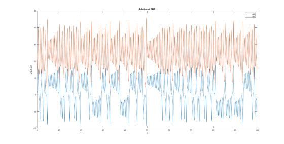
plot(T,x,T,z), xlabel('t'), ylabel('x(t) & z(t)')
title('Solution of ODE'), legend('x(t)', 'z(t)')
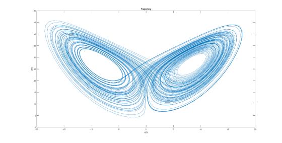
figure, plot(x,z), xlabel('x(t)'), ylabel('z(t)')
title('Trajectory')
function out = dYdt(~, Y)
% Y(1) => x, Y(2) => y, Y(3) = z
out = [-10*Y(1) + 10*Y(2); -Y(1)*Y(3) + 28*Y(1) - Y(2); Y(1)*Y(2) -
8*Y(3)/3];
end
Plots:
Add Answer to:
(Matlab) Use Matlab's built-in Runge-Kutta function ode45 to solve the problem 1010y -xz +28x - y 3 on the interval t є [0, 100 with initial condition (z(0), y(0),z(0)) = (1,1,25), and plot the t...
///MATLAB/// Consider the differential equation over the interval [0,4] with initial condition y(0)=0. 3. Consider the...
 ///MATLAB/// Consider the differential equation over the
interval [0,4] with initial condition y(0)=0.
3. Consider the differential equation n y' = (t3 - t2 -7t - 5)e over the interval [0,4 with initial condition y(0) = 0. (a) Plot the approximate solutions obtained using the methods of Euler, midpoint and the classic fourth order Runge Kutta with n 40 superimposed over the exact solution in the same figure. To plot multiple curves in the same figure, make use of the...
///MATLAB/// Consider the differential equation over the
interval [0,4] with initial condition y(0)=0.
3. Consider the differential equation n y' = (t3 - t2 -7t - 5)e over the interval [0,4 with initial condition y(0) = 0. (a) Plot the approximate solutions obtained using the methods of Euler, midpoint and the classic fourth order Runge Kutta with n 40 superimposed over the exact solution in the same figure. To plot multiple curves in the same figure, make use of the...
use matlab Assignment: 1) Write a function program that implements the 4th Order Runge Kutta Method....
 use
matlab
Assignment: 1) Write a function program that implements the 4th Order Runge Kutta Method. The program must plot each of the k values for each iteration (one plot per k value), and the approximated solution (approximated solution curve). Use the subplot command. There should be a total of five plots. If a function program found on the internet was used, then please cite the source. Show the original program and then show the program after any modifications. Submission...
use
matlab
Assignment: 1) Write a function program that implements the 4th Order Runge Kutta Method. The program must plot each of the k values for each iteration (one plot per k value), and the approximated solution (approximated solution curve). Use the subplot command. There should be a total of five plots. If a function program found on the internet was used, then please cite the source. Show the original program and then show the program after any modifications. Submission...
Solve the following differential equation using MATLAB's ODE45 function. Assume that the all init...
 Solve the following differential equation using MATLAB's ODE45 function. Assume that the all initial conditions are zero and that the input to the system, /(t), is a unit step The output of interest is x dt dt dt To make use of the ODE45 function for this problem, the equation should be expressed in state variable form as shown below Solve the original differential equation for the highest derivative dt 2 dt Assign the following state variables dt dt Express...
Use MATLAB’s ode45 command to solve the following non linear 2nd order ODE: y'' = −y'...
Use MATLAB’s ode45 command to solve the following non linear 2nd order ODE: y'' = −y' + sin(ty) where the derivatives are with respect to time. The initial conditions are y(0) = 1 and y ' (0) = 0. Include your MATLAB code and correctly labelled plot (for 0 ≤ t ≤ 30). Describe the behaviour of the solution. Under certain conditions the following system of ODEs models fluid turbulence over time: dx / dt = σ(y − x) dy...
Can you help me with this problem? This has to be done using Matlab and solving with runge-katta, euler method, and the built in function ode45
 Consider a cylindrical storage tank with surface area A which contains a liquid at depth y:At time t = 0, the tank is empty (y = 0 when t = 0). Liquid is supplied to the tank at a sinusoidal
rate Qin =3Qsin2
(t) and withdrawn from the tank as:
𝑄𝑜𝑢𝑡 = 3(𝑦 − 𝑦𝑜𝑢𝑡)
1.5
if 𝑦 > 𝑦𝑜𝑢𝑡
𝑄𝑜𝑢𝑡 = 0 if 𝑦 ≤ 𝑦𝑜𝑢𝑡 Please note that both 𝑄𝑖𝑛 and 𝑄𝑜𝑢𝑡 have units m3
/h. The mass...
Consider a cylindrical storage tank with surface area A which contains a liquid at depth y:At time t = 0, the tank is empty (y = 0 when t = 0). Liquid is supplied to the tank at a sinusoidal
rate Qin =3Qsin2
(t) and withdrawn from the tank as:
𝑄𝑜𝑢𝑡 = 3(𝑦 − 𝑦𝑜𝑢𝑡)
1.5
if 𝑦 > 𝑦𝑜𝑢𝑡
𝑄𝑜𝑢𝑡 = 0 if 𝑦 ≤ 𝑦𝑜𝑢𝑡 Please note that both 𝑄𝑖𝑛 and 𝑄𝑜𝑢𝑡 have units m3
/h. The mass...
Numerical Methods Consider the following IVP dy=0.01(70-y)(50-y), with y(0)-0 (a) [10 marks Use the Runge-Kutta method of order four to obtain an approximate solution to the ODE at the points t-0.5 an...
 Numerical Methods
Consider the following IVP dy=0.01(70-y)(50-y), with y(0)-0 (a) [10 marks Use the Runge-Kutta method of order four to obtain an approximate solution to the ODE at the points t-0.5 and t1 with a step sizeh 0.5. b) [8 marks Find the exact solution analytically. (c) 7 marks] Use MATLAB to plot the graph of the true and approximate solutions in one figure over the interval [.201. Display graphically the true errors after each steps of calculations.
Consider the...
Numerical Methods
Consider the following IVP dy=0.01(70-y)(50-y), with y(0)-0 (a) [10 marks Use the Runge-Kutta method of order four to obtain an approximate solution to the ODE at the points t-0.5 and t1 with a step sizeh 0.5. b) [8 marks Find the exact solution analytically. (c) 7 marks] Use MATLAB to plot the graph of the true and approximate solutions in one figure over the interval [.201. Display graphically the true errors after each steps of calculations.
Consider the...
MATLAB HELP 3. Consider the equation y′ = y2 − 3x, where y(0) = 1. USE THE EULER AND RUNGE-KUTTA APPROXIMATION SCRIPTS...
 MATLAB HELP 3. Consider the equation y′ = y2 − 3x, where y(0) =
1. USE THE EULER AND RUNGE-KUTTA APPROXIMATION SCRIPTS
PROVIDED IN THE PICTURES
a. Use a Euler approximation with a step size of 0.25 to
approximate y(2).
b. Use a Runge-Kutta approximation with a step size of 0.25 to
approximate y(2).
c. Graph both approximation functions in the same window as a
slope field for the differential equation.
d. Find a formula for the actual solution (not...
MATLAB HELP 3. Consider the equation y′ = y2 − 3x, where y(0) =
1. USE THE EULER AND RUNGE-KUTTA APPROXIMATION SCRIPTS
PROVIDED IN THE PICTURES
a. Use a Euler approximation with a step size of 0.25 to
approximate y(2).
b. Use a Runge-Kutta approximation with a step size of 0.25 to
approximate y(2).
c. Graph both approximation functions in the same window as a
slope field for the differential equation.
d. Find a formula for the actual solution (not...
Solve the following initial value problem using ode45 and ode15s: y",(t) _ Зу"(t) + ty(t) _ sin2(...
 Solve the following initial value problem using ode45 and ode15s: y",(t) _ Зу"(t) + ty(t) _ sin2(t)-7, o s t Plot the solution for varying tolerances. Why do you believe your solution is cor- 2. 1, y(0)-0, y,(0) 1, y"(0)-0. rect?
Solve the following initial value problem using ode45 and ode15s: y",(t) _ Зу"(t) + ty(t) _ sin2(t)-7, o s t Plot the solution for varying tolerances. Why do you believe your solution is cor- 2. 1, y(0)-0, y,(0) 1,...
Solve the following initial value problem using ode45 and ode15s: y",(t) _ Зу"(t) + ty(t) _ sin2(t)-7, o s t Plot the solution for varying tolerances. Why do you believe your solution is cor- 2. 1, y(0)-0, y,(0) 1, y"(0)-0. rect?
Solve the following initial value problem using ode45 and ode15s: y",(t) _ Зу"(t) + ty(t) _ sin2(t)-7, o s t Plot the solution for varying tolerances. Why do you believe your solution is cor- 2. 1, y(0)-0, y,(0) 1,...
Use fourth-order Runge-Kutta method Using MATLAB Solve x - 2t = 0, (0)0,(0) = 0.1, [0, 3] by any convenient method. Gra...
 Use fourth-order Runge-Kutta method
Using MATLAB Solve x - 2t = 0, (0)0,(0) = 0.1, [0, 3] by any convenient method. Graph the solution on
Using MATLAB Solve x - 2t = 0, (0)0,(0) = 0.1, [0, 3] by any convenient method. Graph the solution on
Use fourth-order Runge-Kutta method
Using MATLAB Solve x - 2t = 0, (0)0,(0) = 0.1, [0, 3] by any convenient method. Graph the solution on
Using MATLAB Solve x - 2t = 0, (0)0,(0) = 0.1, [0, 3] by any convenient method. Graph the solution on
MATLAB help please!!!!! 1. Use the forward Euler method Vi+,-Vi + (ti+1-tinti , yi) for i=0.1, 2, , taking yo-y(to) to be the initial condition, to approximate the solution at 2 of the IVP y'=y-t...
 MATLAB help please!!!!!
1. Use the forward Euler method Vi+,-Vi + (ti+1-tinti , yi) for i=0.1, 2, , taking yo-y(to) to be the initial condition, to approximate the solution at 2 of the IVP y'=y-t2 + 1, 0 2, y(0) = 0.5. t Use N 2k, k2,...,20 equispaced timesteps so to 0 and t-1 2) Make a convergence plot computing the error by comparing with the exact solution, y: t (t+1)2 exp(t)/2, and plotting the error as a function of...
MATLAB help please!!!!!
1. Use the forward Euler method Vi+,-Vi + (ti+1-tinti , yi) for i=0.1, 2, , taking yo-y(to) to be the initial condition, to approximate the solution at 2 of the IVP y'=y-t2 + 1, 0 2, y(0) = 0.5. t Use N 2k, k2,...,20 equispaced timesteps so to 0 and t-1 2) Make a convergence plot computing the error by comparing with the exact solution, y: t (t+1)2 exp(t)/2, and plotting the error as a function of...
 ///MATLAB/// Consider the differential equation over the
interval [0,4] with initial condition y(0)=0.
3. Consider the differential equation n y' = (t3 - t2 -7t - 5)e over the interval [0,4 with initial condition y(0) = 0. (a) Plot the approximate solutions obtained using the methods of Euler, midpoint and the classic fourth order Runge Kutta with n 40 superimposed over the exact solution in the same figure. To plot multiple curves in the same figure, make use of the...
///MATLAB/// Consider the differential equation over the
interval [0,4] with initial condition y(0)=0.
3. Consider the differential equation n y' = (t3 - t2 -7t - 5)e over the interval [0,4 with initial condition y(0) = 0. (a) Plot the approximate solutions obtained using the methods of Euler, midpoint and the classic fourth order Runge Kutta with n 40 superimposed over the exact solution in the same figure. To plot multiple curves in the same figure, make use of the...
 use
matlab
Assignment: 1) Write a function program that implements the 4th Order Runge Kutta Method. The program must plot each of the k values for each iteration (one plot per k value), and the approximated solution (approximated solution curve). Use the subplot command. There should be a total of five plots. If a function program found on the internet was used, then please cite the source. Show the original program and then show the program after any modifications. Submission...
use
matlab
Assignment: 1) Write a function program that implements the 4th Order Runge Kutta Method. The program must plot each of the k values for each iteration (one plot per k value), and the approximated solution (approximated solution curve). Use the subplot command. There should be a total of five plots. If a function program found on the internet was used, then please cite the source. Show the original program and then show the program after any modifications. Submission...
 Solve the following differential equation using MATLAB's ODE45 function. Assume that the all initial conditions are zero and that the input to the system, /(t), is a unit step The output of interest is x dt dt dt To make use of the ODE45 function for this problem, the equation should be expressed in state variable form as shown below Solve the original differential equation for the highest derivative dt 2 dt Assign the following state variables dt dt Express...
 Numerical Methods
Consider the following IVP dy=0.01(70-y)(50-y), with y(0)-0 (a) [10 marks Use the Runge-Kutta method of order four to obtain an approximate solution to the ODE at the points t-0.5 and t1 with a step sizeh 0.5. b) [8 marks Find the exact solution analytically. (c) 7 marks] Use MATLAB to plot the graph of the true and approximate solutions in one figure over the interval [.201. Display graphically the true errors after each steps of calculations.
Consider the...
Numerical Methods
Consider the following IVP dy=0.01(70-y)(50-y), with y(0)-0 (a) [10 marks Use the Runge-Kutta method of order four to obtain an approximate solution to the ODE at the points t-0.5 and t1 with a step sizeh 0.5. b) [8 marks Find the exact solution analytically. (c) 7 marks] Use MATLAB to plot the graph of the true and approximate solutions in one figure over the interval [.201. Display graphically the true errors after each steps of calculations.
Consider the...
 MATLAB HELP 3. Consider the equation y′ = y2 − 3x, where y(0) =
1. USE THE EULER AND RUNGE-KUTTA APPROXIMATION SCRIPTS
PROVIDED IN THE PICTURES
a. Use a Euler approximation with a step size of 0.25 to
approximate y(2).
b. Use a Runge-Kutta approximation with a step size of 0.25 to
approximate y(2).
c. Graph both approximation functions in the same window as a
slope field for the differential equation.
d. Find a formula for the actual solution (not...
MATLAB HELP 3. Consider the equation y′ = y2 − 3x, where y(0) =
1. USE THE EULER AND RUNGE-KUTTA APPROXIMATION SCRIPTS
PROVIDED IN THE PICTURES
a. Use a Euler approximation with a step size of 0.25 to
approximate y(2).
b. Use a Runge-Kutta approximation with a step size of 0.25 to
approximate y(2).
c. Graph both approximation functions in the same window as a
slope field for the differential equation.
d. Find a formula for the actual solution (not...
 Solve the following initial value problem using ode45 and ode15s: y",(t) _ Зу"(t) + ty(t) _ sin2(t)-7, o s t Plot the solution for varying tolerances. Why do you believe your solution is cor- 2. 1, y(0)-0, y,(0) 1, y"(0)-0. rect?
Solve the following initial value problem using ode45 and ode15s: y",(t) _ Зу"(t) + ty(t) _ sin2(t)-7, o s t Plot the solution for varying tolerances. Why do you believe your solution is cor- 2. 1, y(0)-0, y,(0) 1,...
Solve the following initial value problem using ode45 and ode15s: y",(t) _ Зу"(t) + ty(t) _ sin2(t)-7, o s t Plot the solution for varying tolerances. Why do you believe your solution is cor- 2. 1, y(0)-0, y,(0) 1, y"(0)-0. rect?
Solve the following initial value problem using ode45 and ode15s: y",(t) _ Зу"(t) + ty(t) _ sin2(t)-7, o s t Plot the solution for varying tolerances. Why do you believe your solution is cor- 2. 1, y(0)-0, y,(0) 1,...
 Use fourth-order Runge-Kutta method
Using MATLAB Solve x - 2t = 0, (0)0,(0) = 0.1, [0, 3] by any convenient method. Graph the solution on
Using MATLAB Solve x - 2t = 0, (0)0,(0) = 0.1, [0, 3] by any convenient method. Graph the solution on
Use fourth-order Runge-Kutta method
Using MATLAB Solve x - 2t = 0, (0)0,(0) = 0.1, [0, 3] by any convenient method. Graph the solution on
Using MATLAB Solve x - 2t = 0, (0)0,(0) = 0.1, [0, 3] by any convenient method. Graph the solution on
 MATLAB help please!!!!!
1. Use the forward Euler method Vi+,-Vi + (ti+1-tinti , yi) for i=0.1, 2, , taking yo-y(to) to be the initial condition, to approximate the solution at 2 of the IVP y'=y-t2 + 1, 0 2, y(0) = 0.5. t Use N 2k, k2,...,20 equispaced timesteps so to 0 and t-1 2) Make a convergence plot computing the error by comparing with the exact solution, y: t (t+1)2 exp(t)/2, and plotting the error as a function of...
MATLAB help please!!!!!
1. Use the forward Euler method Vi+,-Vi + (ti+1-tinti , yi) for i=0.1, 2, , taking yo-y(to) to be the initial condition, to approximate the solution at 2 of the IVP y'=y-t2 + 1, 0 2, y(0) = 0.5. t Use N 2k, k2,...,20 equispaced timesteps so to 0 and t-1 2) Make a convergence plot computing the error by comparing with the exact solution, y: t (t+1)2 exp(t)/2, and plotting the error as a function of...
Most questions answered within 3 hours.
-
Hastings Entertainment has a beta of 0.64. If the market return
is expected to be 13.80...
asked 5 minutes ago -
9. Depository institutions are always:
a. illiquid
b. profitable
c. insolvent
d. all of the above...
asked 13 minutes ago -
Use AstroTurf Company's income statement below to answer the
following two questions. Answer these questions with...
asked 13 minutes ago -
How is a firm's task
environment different from its general environment? Provide
examples of both types...
asked 11 minutes ago -
What is one reason Innovators can adopt innovations so
early?
Group of answer choices
they are...
asked 13 minutes ago -
Show that min x^2, s.t. x>=2 has strong duality.
asked 14 minutes ago -
Using curved arrows show how the intermediate formed in this
reaction (Hexaphenylbenzene is prepared through a...
asked 19 minutes ago -
Two lightbulbs operate on the same current. Bulb A has four
times the power output of...
asked 16 minutes ago -
1. What five (5) basic parameters need to be measured
during a pump test in order...
asked 27 minutes ago -
One student ran a TLC of an unknown compound on a
silica gel plate and the...
asked 30 minutes ago -
Use inheritance to create a new class AudioRecording
based on Recording class that:
it will retain...
asked 35 minutes ago -
In the long run, an increase in the quantity of money ________
the value of money...
asked 41 minutes ago