
Homework Answers
Add Answer to:
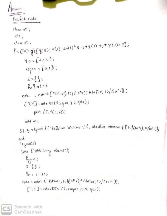
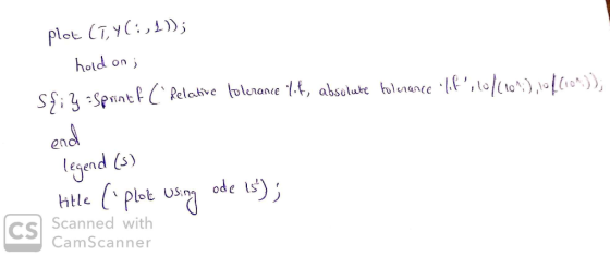
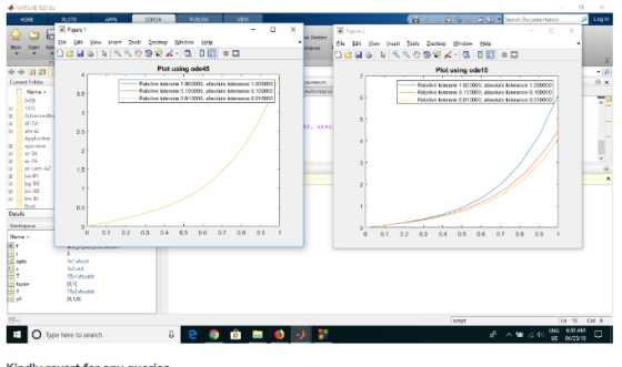
Solve the following initial value problem using ode45 and ode15s: y",(t) _ Зу"(t) + ty(t) _ sin2(...
Solve the initial value problem dt y+e' a. Use ode45() to find the approximate values of...
 Solve the initial value problem dt y+e' a. Use ode45() to find the approximate values of the solution at 1-0,1,1.8,2.1 and also plot the solution. Now plot the numerical solution of several large intervals and make a guess about the nature of the solution as t b.
Solve the initial value problem ty' + 2ty = 3t + 4, y(1)=theta and plot y...
 Solve the initial value problem ty' + 2ty = 3t + 4, y(1)=theta and plot y versus t for t in the interval [1/2., 2] using matlab.
(Matlab) Use Matlab's built-in Runge-Kutta function ode45 to solve the problem 1010y -xz +28x - y 3 on the interval t є [0, 100 with initial condition (z(0), y(0),z(0)) = (1,1,25), and plot the t...
 (Matlab) Use Matlab's built-in Runge-Kutta function ode45 to solve the problem 1010y -xz +28x - y 3 on the interval t є [0, 100 with initial condition (z(0), y(0),z(0)) = (1,1,25), and plot the trajectory of the solution ((t), (t)) forte [0, 100
(Matlab) Use Matlab's built-in Runge-Kutta function ode45 to solve the problem 1010y -xz +28x - y 3 on the interval t є [0, 100 with initial condition (z(0), y(0),z(0)) = (1,1,25), and plot the trajectory of the...
(Matlab) Use Matlab's built-in Runge-Kutta function ode45 to solve the problem 1010y -xz +28x - y 3 on the interval t є [0, 100 with initial condition (z(0), y(0),z(0)) = (1,1,25), and plot the trajectory of the solution ((t), (t)) forte [0, 100
(Matlab) Use Matlab's built-in Runge-Kutta function ode45 to solve the problem 1010y -xz +28x - y 3 on the interval t є [0, 100 with initial condition (z(0), y(0),z(0)) = (1,1,25), and plot the trajectory of the...
Use MATLAB’s ode45 command to solve the following non linear 2nd order ODE: y'' = −y'...
Use MATLAB’s ode45 command to solve the following non linear 2nd order ODE: y'' = −y' + sin(ty) where the derivatives are with respect to time. The initial conditions are y(0) = 1 and y ' (0) = 0. Include your MATLAB code and correctly labelled plot (for 0 ≤ t ≤ 30). Describe the behaviour of the solution. Under certain conditions the following system of ODEs models fluid turbulence over time: dx / dt = σ(y − x) dy...
(1 point) Solve the initial value problem ty" - ty' y = 5, y(0) = 5,...
 (1 point) Solve the initial value problem ty" - ty' y = 5, y(0) = 5, y'(0) = -1 y =
Solve for Y(s), the Laplace transform of the solution y(t) to the initial value problem below....
 Solve for Y(s), the Laplace transform of the solution y(t) to the initial value problem below. y" + 4y = 512 - 2. y(0)=0, 7(0) = -8 Click here to view the table of Laplace transforms Click here to view the table of properties of Laplace transforms. Solve for Y(s), the Laplace transform of the solution y(t) to the initial value problem below. y" + 4y = 5t2 - 2. y(0) = 0, y'(O) = - 8 Click here to...
Solve initial value problem using Laplace transform Problem 4 Solve the initial value problems given below...
 Solve initial value problem using Laplace transform
Problem 4 Solve the initial value problems given below --ез, y(0) 2. a. b. f ty 3 cos t, y(0)-
Solve initial value problem using Laplace transform
Problem 4 Solve the initial value problems given below --ез, y(0) 2. a. b. f ty 3 cos t, y(0)-
Solve the following differential equation using MATLAB's ODE45 function. Assume that the all init...
 Solve the following differential equation using MATLAB's ODE45 function. Assume that the all initial conditions are zero and that the input to the system, /(t), is a unit step The output of interest is x dt dt dt To make use of the ODE45 function for this problem, the equation should be expressed in state variable form as shown below Solve the original differential equation for the highest derivative dt 2 dt Assign the following state variables dt dt Express...
IN PYTHON: 6. Stiff Problem Consider the initial value problem y = -500(y - cost) -...
 IN PYTHON:
6. Stiff Problem Consider the initial value problem y = -500(y - cost) - sint, to= 0, yo = 2. Recall from class that the problem is stiff. Solve it with the explicit RK45 and implicit Radau in the module scipy.integrate up to time T = 1 and the default tolerances. 1. Plot the solution. 2. Print the number of steps of each method. 3. Print the difference between the methods at the final time T.
IN PYTHON:
6. Stiff Problem Consider the initial value problem y = -500(y - cost) - sint, to= 0, yo = 2. Recall from class that the problem is stiff. Solve it with the explicit RK45 and implicit Radau in the module scipy.integrate up to time T = 1 and the default tolerances. 1. Plot the solution. 2. Print the number of steps of each method. 3. Print the difference between the methods at the final time T.
7. Solve the initial value problem --( y = -1 00 when the initial value is...
 7. Solve the initial value problem --( y = -1 00 when the initial value is given as following: and discuss the behavior of the solution as t (you may sketch the solution curve.) (a) X(0) = (0,0.5).
7. Solve the initial value problem --( y = -1 00 when the initial value is given as following: and discuss the behavior of the solution as t (you may sketch the solution curve.) (a) X(0) = (0,0.5).
7. Solve the initial value problem --( y = -1 00 when the initial value is given as following: and discuss the behavior of the solution as t (you may sketch the solution curve.) (a) X(0) = (0,0.5).
 Solve the initial value problem dt y+e' a. Use ode45() to find the approximate values of the solution at 1-0,1,1.8,2.1 and also plot the solution. Now plot the numerical solution of several large intervals and make a guess about the nature of the solution as t b.
 Solve the initial value problem ty' + 2ty = 3t + 4, y(1)=theta and plot y versus t for t in the interval [1/2., 2] using matlab.
 (Matlab) Use Matlab's built-in Runge-Kutta function ode45 to solve the problem 1010y -xz +28x - y 3 on the interval t є [0, 100 with initial condition (z(0), y(0),z(0)) = (1,1,25), and plot the trajectory of the solution ((t), (t)) forte [0, 100
(Matlab) Use Matlab's built-in Runge-Kutta function ode45 to solve the problem 1010y -xz +28x - y 3 on the interval t є [0, 100 with initial condition (z(0), y(0),z(0)) = (1,1,25), and plot the trajectory of the...
(Matlab) Use Matlab's built-in Runge-Kutta function ode45 to solve the problem 1010y -xz +28x - y 3 on the interval t є [0, 100 with initial condition (z(0), y(0),z(0)) = (1,1,25), and plot the trajectory of the solution ((t), (t)) forte [0, 100
(Matlab) Use Matlab's built-in Runge-Kutta function ode45 to solve the problem 1010y -xz +28x - y 3 on the interval t є [0, 100 with initial condition (z(0), y(0),z(0)) = (1,1,25), and plot the trajectory of the...
 (1 point) Solve the initial value problem ty" - ty' y = 5, y(0) = 5, y'(0) = -1 y =
 Solve for Y(s), the Laplace transform of the solution y(t) to the initial value problem below. y" + 4y = 512 - 2. y(0)=0, 7(0) = -8 Click here to view the table of Laplace transforms Click here to view the table of properties of Laplace transforms. Solve for Y(s), the Laplace transform of the solution y(t) to the initial value problem below. y" + 4y = 5t2 - 2. y(0) = 0, y'(O) = - 8 Click here to...
 Solve initial value problem using Laplace transform
Problem 4 Solve the initial value problems given below --ез, y(0) 2. a. b. f ty 3 cos t, y(0)-
Solve initial value problem using Laplace transform
Problem 4 Solve the initial value problems given below --ез, y(0) 2. a. b. f ty 3 cos t, y(0)-
 Solve the following differential equation using MATLAB's ODE45 function. Assume that the all initial conditions are zero and that the input to the system, /(t), is a unit step The output of interest is x dt dt dt To make use of the ODE45 function for this problem, the equation should be expressed in state variable form as shown below Solve the original differential equation for the highest derivative dt 2 dt Assign the following state variables dt dt Express...
 IN PYTHON:
6. Stiff Problem Consider the initial value problem y = -500(y - cost) - sint, to= 0, yo = 2. Recall from class that the problem is stiff. Solve it with the explicit RK45 and implicit Radau in the module scipy.integrate up to time T = 1 and the default tolerances. 1. Plot the solution. 2. Print the number of steps of each method. 3. Print the difference between the methods at the final time T.
IN PYTHON:
6. Stiff Problem Consider the initial value problem y = -500(y - cost) - sint, to= 0, yo = 2. Recall from class that the problem is stiff. Solve it with the explicit RK45 and implicit Radau in the module scipy.integrate up to time T = 1 and the default tolerances. 1. Plot the solution. 2. Print the number of steps of each method. 3. Print the difference between the methods at the final time T.
 7. Solve the initial value problem --( y = -1 00 when the initial value is given as following: and discuss the behavior of the solution as t (you may sketch the solution curve.) (a) X(0) = (0,0.5).
7. Solve the initial value problem --( y = -1 00 when the initial value is given as following: and discuss the behavior of the solution as t (you may sketch the solution curve.) (a) X(0) = (0,0.5).
7. Solve the initial value problem --( y = -1 00 when the initial value is given as following: and discuss the behavior of the solution as t (you may sketch the solution curve.) (a) X(0) = (0,0.5).
Most questions answered within 3 hours.
-
You have a 825.3 mL sample of 2.754 M HA (Ka =
4.49⋅10−4). Calculate the pH...
asked 10 minutes ago -
The blues made its way into many kinds of music. Eric Clapton,
The Beatles, and Elvis...
asked 2 hours ago -
8. A wave in a string has a wave function given by: y (x, t) =...
asked 1 hour ago -
If you’re standing at the bottom of a hill and asked to evaluate
it while being...
asked 3 hours ago -
1. Which region has taken the lead in the world of
e-waste handling?
a) European Union...
asked 3 hours ago -
A 8.15- g bullet from a 9-mm pistol has a velocity of 366.0 m/s.
It strikes...
asked 4 hours ago -
The outstanding bonds of Alpha Extracts have a yield to maturity
of 7.4 percent and a...
asked 4 hours ago -
The Problem: The Case of the Harmonizing Vacations
Your CEO is exploring partnering with a European...
asked 5 hours ago -
A chemical equation is balanced by adding coefficients in front
of some formulas so that the...
asked 5 hours ago -
From the literature (reference your sources): What are the
lattice parameters of calcite and aragonite? Why...
asked 6 hours ago -
Your system is rejecting the question am asking which is
preceded by a case study. It...
asked 6 hours ago -
3. On January 2, 2000, Larry creates a trust with himself as
trustee. Larry as trustee...
asked 6 hours ago