

A real estate developer wishes to study the relationship between the size of home a client will purchase (in square feet) and other variables. Possible independent variables include the family income, family size, whether there is a senior adult parent living with the family (1 for yes, 0 for no), and the total years of education beyond high school for the husband and wife. The sample information is reported below Square Income Family Senior Family Feet (000s) Size Parent Education 60.8 2,380 68.4 3,640 104.5 3,360 89.3 3,080 2,940 72.2 10 4,480 1254 83.6 133 2,520 4.200 10 2,800 95 a. Develop an appropriate mutiple regression equation using stopwise method. (Use Excel data analysis and enter number of family members first, then their income and delete any insignificant variables. Leave no cells blank be certain to enter "0" wherever required. Round your answers to 2 decimal places.) Step Family T-Value P-Value b. Select all independent variables that should be in the final model. (Select all that apply.) Senior parent Square feet Family size Income Education
Homework Answers
1)
First, the data is entered in Excel:
| Sales | Ad_Dollars | Accounts | Competitors | Potential |
| 79.3 | 5.5 | 31 | 10 | 8 |
| 200.1 | 2.5 | 55 | 8 | 6 |
| 163.2 | 8 | 67 | 12 | 9 |
| 200.1 | 3 | 50 | 7 | 16 |
| 146 | 3 | 38 | 8 | 15 |
| 177.7 | 2.9 | 71 | 12 | 17 |
| 30.9 | 8 | 30 | 12 | 8 |
| 291.9 | 9 | 56 | 5 | 10 |
| 160 | 4 | 42 | 8 | 4 |
| 339.4 | 6.5 | 73 | 5 | 16 |
| 159.6 | 5.5 | 60 | 11 | 7 |
| 86.3 | 5 | 44 | 12 | 12 |
| 237.5 | 6 | 50 | 6 | 6 |
| 107.2 | 5 | 39 | 10 | 4 |
| 155 | 3.5 | 55 | 10 | 4 |
| 291.4 | 8 | 70 | 6 | 14 |
| 100.2 | 6 | 40 | 11 | 6 |
| 135.8 | 4 | 50 | 11 | 8 |
| 223.3 | 7.5 | 62 | 9 | 13 |
| 195 | 7 | 59 | 9 | 11 |
| 73.4 | 6.7 | 53 | 13 | 5 |
| 47.7 | 6.1 | 38 | 13 | 10 |
| 140.7 | 3.6 | 43 | 9 | 17 |
| 93.5 | 4.2 | 26 | 8 | 3 |
| 259 | 4.5 | 75 | 8 | 19 |
| 331.2 | 5.6 | 71 | 4 | 9 |
The data is first visualized through a matrix of scatterplots:
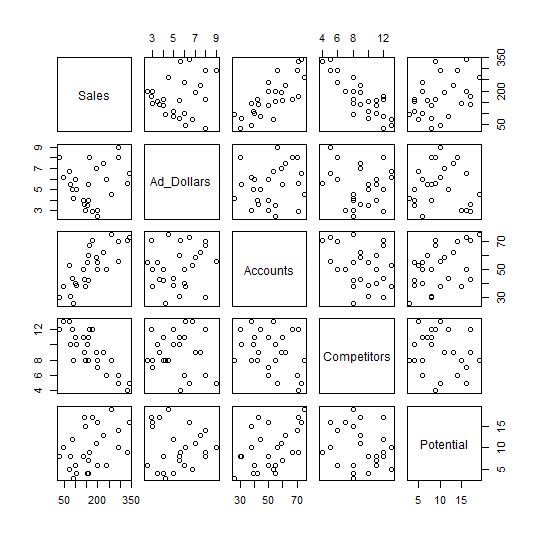
The above diagram shows that the Sales is weakly correlated with Ad Dollars and mildly with Potential, positively correlated with Accounts, and negatively correlated with Competitors. We first build a linear model as function of all variables:
> tt <- read.csv("clipboard",header=TRUE,sep="\t")
> pairs(tt)
> sales_lm <- lm(Sales~.,tt)
> summary(sales_lm)
Call:
lm(formula = Sales ~ ., data = tt)
Residuals:
Min
1Q Median
3Q Max
-19.0906 -5.9796 0.8968 6.5667 14.7985
Coefficients:
Estimate Std. Error t value Pr(>|t|)
(Intercept) 178.3203 12.9603 13.759 5.62e-12
***
Ad_Dollars 1.8071
1.0810 1.672
0.109
Accounts
3.3178 0.1629 20.368 2.60e-15 ***
Competitors -21.1850 0.7879 -26.887 <
2e-16 ***
Potential 0.3245
0.4678 0.694
0.495
---
Signif. codes: 0 ‘***’ 0.001 ‘**’ 0.01 ‘*’ 0.05 ‘.’ 0.1 ‘ ’ 1
Residual standard error: 9.604 on 21 degrees of freedom
Multiple R-squared: 0.9892, Adjusted R-squared:
0.9871
F-statistic: 479.1 on 4 and 21 DF, p-value: < 2.2e-16
The model is significant, and the covariates Accounts and Potential are significant variables.
The overall elasticity is 40.68815.
>
predict(sales_lm,newdata=list(Ad_Dollars=8,Accounts=30,Competitors=12,Potential=8)
+ )
1
40.68815
2)
a)
|
family |
square feet |
income |
family size |
senior parent |
parent education |
|
1 |
2240 |
60.8 |
2 |
0 |
4 |
|
2 |
2380 |
68.4 |
2 |
1 |
6 |
|
3 |
3640 |
104.5 |
3 |
0 |
7 |
|
4 |
3360 |
89.3 |
1 |
1 |
0 |
|
5 |
3080 |
72.2 |
4 |
0 |
2 |
|
6 |
2940 |
114.3 |
1 |
1 |
10 |
|
7 |
4480 |
125.4 |
6 |
0 |
6 |
|
8 |
2520 |
83.6 |
3 |
0 |
8 |
|
9 |
4200 |
133.5 |
5 |
0 |
2 |
|
10 |
2800 |
95.3 |
3 |
0 |
6 |
Regression Analysis: square feet versus income family ....nt, Education
Stepwise selection of terms
α to enter = 0.15, α to remove = 0.15
Analysis of Variance
Source DF Adj SS Adj MS F-value P-value
Regression 2 4619699 2309849 30.90 0.000
income 1 380692 380692 5.09 0.059
family size 1 962595 962595 12.88 0.009
Error 7 523341 74763
Total 9 5143040
Model Summary
S R-sq R-sq(adj) R-sq(pred)
273.428 89.82% 86.92% 82.48%
Coefficients
Term Coef SE Coef T-value p-value VIF
Constant 713 363 1.96 0.091
income 12.15 5.38 2.26 0.0059 2.08
family size 372 104 3.59 0.009 2.08
Regression Equation
Square feet = 713 + 12.15 income + 372 family size
Fits and Diagnostics for Unusual Observations
Obs Square feet fit Resid Std Resid
3 3640 3098 542 2.25 R
R large residual
From the above output, the multiple linear regression equation is,
Y = 713 + 12.15 (income, X1) + 372 (Family size, X2)
b)
Family size and income are independent variables. That should be in the final model.
Add Answer to:
Great Plains Roofing and Siding Company Inc. sells roofing and siding products to home repair retailers, such...
A real estate developer wishes to study the relationship between the size of home a client will purchase (in square...
 A real estate developer wishes to study the relationship between the size of home a client will purchase (in square feet) and other variables. Possible independent variables include the family income, family size, whether there is a senior adult parent living with the family (1 for yes, 0 for no), and the total years of education beyond high school for the husband and wife. The sample information is reported below Square Income Family Senior Family Feet (000s) Size Parent Education...
A real estate developer wishes to study the relationship between the size of home a client...
 A real estate developer wishes to study the relationship between the size of home a client will purchase (in square feet) and other variables. Possible independent variables include the family income, family size, whether there is a senior adult parent living with the family (1 for yes, O for no), and the total years of education beyond high school for the husband and wife. The sample information is reported below. Family Size Senior Parent Education Family Square Feet 2,300 2,300...
SUMMARY OUTPUT 0.865 0.748 Regression Statistics Multiple R R Square Adjusted R Square Standard Error Observations...
 SUMMARY OUTPUT 0.865 0.748 Regression Statistics Multiple R R Square Adjusted R Square Standard Error Observations 0.726 5.195 50 ANOVA df SS MS F Significance F 0.0000 3605.7736 1201.9245 Regression Residual Total 1214.2264 26.3962 49 4820 P-value 0.7798 Intercept Income Coefficients Standard Error -1.6335 5.8078 0.4485 0.1137 4.2615 0.8062 -0.6517 0.4319 t Stat -0.281 3.9545 0.0003 Size 5.286 0.0001 0.1383 School -1.509 A real estate builder wishes to determine how house size (House) is influenced by family income (Income). family...
All Greens is a franchise store that sells house plants and lawn and garden supplies. Although Al...
All Greens is a franchise store that sells house plants and lawn and garden supplies. Although All Greens is a franchise, each store is owned and managed by private individuals. Some friends have asked you to go into business with them to open a new All Greens store in the suburbs of San Diego. The national franchise headquarters sent you the following information at your request. These data are about 27 All Greens stores in California. Each of the 27...
Al Greens is a franchise store that sells house plants and lawn and garden supplies. Although...
 Al Greens is a franchise store that sells house plants and lawn and garden supplies. Although Al Greens is a franchise, each store is owned and managed by private individuals. Some friends have asked you to go into business with them to open a new All Greens store in the suburbs of San Diego. The national franchise headquarters sent you the following information at your request. These data are about 27 Al Greens stores in California. Each of the 27...
All Greens is a franchise store that sells house plants and lawn and garden supplies. Although All Greens is a franchise, each store is owned and managed by private individuals. Some friends have aske...
All Greens is a franchise store that sells house plants and lawn and garden supplies. Although All Greens is a franchise, each store is owned and managed by private individuals. Some friends have asked you to go into business with them to open a new All Greens store in the suburbs of San Diego. The national franchise headquarters sent you the following information at your request. These data are about 27 All Greens stores in California. Each of the 27...
Hi I need help with these questions on Excel for linear regression! Gulf Home Data Price...
Hi I need help with these questions on Excel for linear regression! Gulf Home Data Price Size Number of Niceness Pool? Home ($1000s) (Square Feet) Bathrooms Rating yes=1; no=0 This information is taken from 80 homes recently sold 1 260.9 2666 2.5 7 0 along the Gulf of Mexico coast. You are to analyze 2 337.3 3418 3.5 6 1 the data to discover which of the variables have a 3 268.4 2945 2.0 5 1 statistically...
The following ANOVA model is for a multiple regression model with two independent variables: Degrees of Sum of Mean Source Freedom Squares ...
 The following ANOVA model is for a multiple regression model
with two independent variables:
Degrees
of
Sum
of
Mean
Source
Freedom
Squares
Squares
F
Regression
2
60
Error
18
120
Total
20
180
Determine the Regression Mean Square (MSR):
Determine the Mean Square Error (MSE):
Compute the overall Fstat test statistic.
Is the Fstat significant at the 0.05 level?
A linear regression was run on auto sales relative to consumer
income. The Regression Sum of Squares (SSR) was 360 and...
The following ANOVA model is for a multiple regression model
with two independent variables:
Degrees
of
Sum
of
Mean
Source
Freedom
Squares
Squares
F
Regression
2
60
Error
18
120
Total
20
180
Determine the Regression Mean Square (MSR):
Determine the Mean Square Error (MSE):
Compute the overall Fstat test statistic.
Is the Fstat significant at the 0.05 level?
A linear regression was run on auto sales relative to consumer
income. The Regression Sum of Squares (SSR) was 360 and...
Compute the cost of a single preschool class and a single birthday party using the current...
 Compute the cost of a single preschool class and a single
birthday party using the current cost system.
Introduction Tots R Us (TRU) had been running a small, for-profit preschool program for young children between the ages of two and four for several decades. TRU was one of several privately run programs in the suburban Boston area. For each of the three age groups i.e., two-, three- and four-year olds), there were two classes per day for a total of...
Compute the cost of a single preschool class and a single
birthday party using the current cost system.
Introduction Tots R Us (TRU) had been running a small, for-profit preschool program for young children between the ages of two and four for several decades. TRU was one of several privately run programs in the suburban Boston area. For each of the three age groups i.e., two-, three- and four-year olds), there were two classes per day for a total of...
Introduction Young School for Wee People Young School for Wee People (YSWP) had been running a...
Introduction Young School for Wee People Young School for Wee People (YSWP) had been running a small, for-profit preschool program for young children between the ages of two and four for several decades. YSWP was one of several privately run programs in the suburban Philadelphia area. For each of the three age groups (i.e., two-, three- and four-year olds), there were two classes per day for a total of six classes in the facility each day. The classes were held...
 A real estate developer wishes to study the relationship between the size of home a client will purchase (in square feet) and other variables. Possible independent variables include the family income, family size, whether there is a senior adult parent living with the family (1 for yes, 0 for no), and the total years of education beyond high school for the husband and wife. The sample information is reported below Square Income Family Senior Family Feet (000s) Size Parent Education...
 A real estate developer wishes to study the relationship between the size of home a client will purchase (in square feet) and other variables. Possible independent variables include the family income, family size, whether there is a senior adult parent living with the family (1 for yes, O for no), and the total years of education beyond high school for the husband and wife. The sample information is reported below. Family Size Senior Parent Education Family Square Feet 2,300 2,300...
 SUMMARY OUTPUT 0.865 0.748 Regression Statistics Multiple R R Square Adjusted R Square Standard Error Observations 0.726 5.195 50 ANOVA df SS MS F Significance F 0.0000 3605.7736 1201.9245 Regression Residual Total 1214.2264 26.3962 49 4820 P-value 0.7798 Intercept Income Coefficients Standard Error -1.6335 5.8078 0.4485 0.1137 4.2615 0.8062 -0.6517 0.4319 t Stat -0.281 3.9545 0.0003 Size 5.286 0.0001 0.1383 School -1.509 A real estate builder wishes to determine how house size (House) is influenced by family income (Income). family...
 Al Greens is a franchise store that sells house plants and lawn and garden supplies. Although Al Greens is a franchise, each store is owned and managed by private individuals. Some friends have asked you to go into business with them to open a new All Greens store in the suburbs of San Diego. The national franchise headquarters sent you the following information at your request. These data are about 27 Al Greens stores in California. Each of the 27...
 The following ANOVA model is for a multiple regression model
with two independent variables:
Degrees
of
Sum
of
Mean
Source
Freedom
Squares
Squares
F
Regression
2
60
Error
18
120
Total
20
180
Determine the Regression Mean Square (MSR):
Determine the Mean Square Error (MSE):
Compute the overall Fstat test statistic.
Is the Fstat significant at the 0.05 level?
A linear regression was run on auto sales relative to consumer
income. The Regression Sum of Squares (SSR) was 360 and...
The following ANOVA model is for a multiple regression model
with two independent variables:
Degrees
of
Sum
of
Mean
Source
Freedom
Squares
Squares
F
Regression
2
60
Error
18
120
Total
20
180
Determine the Regression Mean Square (MSR):
Determine the Mean Square Error (MSE):
Compute the overall Fstat test statistic.
Is the Fstat significant at the 0.05 level?
A linear regression was run on auto sales relative to consumer
income. The Regression Sum of Squares (SSR) was 360 and...
 Compute the cost of a single preschool class and a single
birthday party using the current cost system.
Introduction Tots R Us (TRU) had been running a small, for-profit preschool program for young children between the ages of two and four for several decades. TRU was one of several privately run programs in the suburban Boston area. For each of the three age groups i.e., two-, three- and four-year olds), there were two classes per day for a total of...
Compute the cost of a single preschool class and a single
birthday party using the current cost system.
Introduction Tots R Us (TRU) had been running a small, for-profit preschool program for young children between the ages of two and four for several decades. TRU was one of several privately run programs in the suburban Boston area. For each of the three age groups i.e., two-, three- and four-year olds), there were two classes per day for a total of...
Most questions answered within 3 hours.
-
At the beginning of the period, the Fabricating Department
budgeted direct labor of $136,500 and equipment...
asked 46 seconds ago -
PARTS A-D HAVE BEEN ANSWERED. WAS TOLD TO REPOST. ONLY ANSWER
PARTS E and F.
A...
asked 18 minutes ago -
2) You are given the task of finding a representation for a
circle in a drawing...
asked 1 hour ago -
STUDY QUESTION: Does use of diet drug fen-phen
(fenfluramine-phentermine) cause valvular heart disease?
HINT: Valvular heart...
asked 1 hour ago -
1. An object weighing 40 N rests on a surface. The coefficient
of friction is 0.35....
asked 2 hours ago -
Investor company owns 35% of investee company voting stock and
accounts for the investment under the...
asked 3 hours ago -
The number of major faults on a randomly chosen 1 km stretch of
highway has a...
asked 4 hours ago -
Consider the competitive environment of Starbuck's, Progressive
Insurance, a manufacturing firm with low turnover, or a...
asked 4 hours ago -
3. Gains from trade
Consider two neighbouring island countries called Euphoria and
Contente. They each have...
asked 6 hours ago -
A business executive has the option to invest money in two
plans: Plan A guarantees that...
asked 9 hours ago -
Hello, can someone please help me answer this question?
How much heat is absorbed by a...
asked 9 hours ago -
. A marketing researcher conducted a survey of 25 shoppers
randomly selected at the local mall...
asked 9 hours ago