Question

This is taken from Section 4.6, "Amplitude Modulation and the Continuous-Time Fourier Transform," in the course text Computer Explorations in signals and systems by Buck, Daniel, Singer, 2nd Edition. I need the answers for the basic and intermediate questions.

4.6 Amplitude Modulation and the Continuous-Time Fouriei Transform This exercise will explore amplitude modulation of Morse code messages. A simple ampli tude modulation system can be described by x(t) = m(t) cos(Crfot), (4.13) where m(t) is called the message waveform and fo is the modulation frequency. The continuous-time Fourier transform (CTFT) of a cosine of frequency fo is (4.14) which can confirmed by substituting C(j) into Eq. 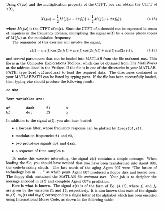(4.1) to yield (4.15) cos(2T fot)- Using C(ju) and the multiplication property of the CTFT, you can obtain the CTFT of r(t) (4.16) where M(ju) is the CTFT of m(t). Since the CTFT of a sinusoid can be expressed in terms of impulses in the frequency domain, multiplying the signal m(t) by a cosine places copies of M(jw) at the modulation frequency The remainder of this exercise will involve the signal, r(t)m(t) cos(2 fit) +m2(t) cos(2 f2t) ma(t) sin(2fit) and several parameters that can be loaded into MATLAB from the file ctftmod.mat. This file is in the Computer Explorations Toolbox, which can be obtained from The MathWorks at the address listed in the Preface. If the file is in one of the directories in your MATLAB PATH, type load ctftmod.mat to load the required data. The directories contained in your MATLABPATH can be listed by typing path. If the file has been successfully loaded, then typing who should produce the following result: >>who Your variables are: af dash bf dot f2 In addition to the signal r(t), you also have loaded: . a lowpass filter, whose frequency response can be plotted by freqs (bf,af), modulation frequencies f1 and f2, two prototype signals dot and dash, a sequence of time samples t To make this exercise interesting, the signal z(t) contains a simple message. When loading the file, you should have noticed that you have been transformed into Agent 008, the code-breaking sleuth. The last words of the aging Agent 007 were "The future of technology lies in" at which point Agent 007 produced a floppy disk and keeled over The floppy disk contained the MATLAB file ctftmod.mat. Your job is to decipher the message encoded in z(t) and complete Agent 007's prediction. Here is what is known. The signal z(t) is of the form of Eq. (4.17), where fi and f are given by the ariables f1 and f2, respectively. It is also known that each of the signals mi (t), m2(t) and m(t) correspond to a single letter of the alphabet which has been encoded using International Morse Code, as shown in the following table: Basic Problems (a). Using the signals dot and dash, construct the signal that corresponds to the letter Z' in Morse code, and plot it against t. As an example, the letter C is constructed by typing c-[dash dot dash dot]. Store your signal z(t) in the vector z. (b). Plot the frequency response of the filter using freqs (bf,af) (c). The signals dot and dash are each composed of low frequency components such that their Fourier transforms lie roughly within the passband of the lowpass filter. Demon- strate this by filtering each of the two signals using >> ydash-lsim(bf,af,dash, t (1:length(dash))) > ydot-lsim(bf,af,dot,t (1:length (dot))); Plot the outputs ydash and ydot along with the original signals dash and dot (d). When the signal dash is modulated by cos(2m fit), most of the energy in the Fourier transform wil move outside the passband of the filter. Create the signal y(t) by executing y-dash*cos(2 pi fi t1length (dash)). Plot the signal gy(t) Also plot the output yo-lsim (bf,af,y,t). Do you get a result that you would have expected? Intermediate Problems (e). Determine analytically the Fourier transform of each of the signals m(t) cos(2T fit) cos(2 fit) m(t) cos(2fit) sin(2nfit) and m(t) cos(2T fit) cos(2m f2t), in terms of M(jw), the Fourier transform of m(t) (f). Using your results from Part (e) and by examining the frequency response of the filter as plotted in Part (b), devise a plan for extracting the signalrn1(t) from (t). Plot the signal mi(t) and determine which letter is represented in Morse code by the signal. (g). Repeat Part (f) for the signals m2(t) and m(t). Agent 008, where does the future of technology lie?

Answer 1

at node (a): 11-16 12 ^-2A apply keu at node Cb) Kcu at a 2-o Zy:-2月 fpplykeL at node. CC) . 5-t-