Question

Show work if possible please

An experiment has a single factor with five groups and five values in each group. freedom. In determining the total variation, there are: determining the among-group variation, there are 4 degrees freedom. In determining the within-group variation, there are 20 degrees of degrees of freedom. Also, note that SSA 96, SsW 120, SST = 216, MSA 24. MSW 6, and FSTAT 4. Complete parts (a) through (d). Click here to view page 1 of the F table. Click here to view page 2 of the F table. Click here view page 3 of the F table. Click here to view page 4 of the F table. Construct the ANOVA summary table and fill in all values the table. Degrees of Freedom Sum of Mean Square (Variance) F Source Squares Among groups Within groups Total (Simplify your answers.) At the 0.005 level of significance, what is the upper-tail critical value from the F distribution? 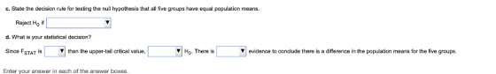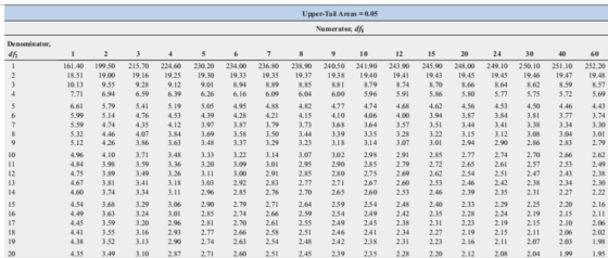Fo.005 (Round to two decimal places as needed.) c. State the decision rule for testing the null hypothesis that all five groups have equal population means. Reject Ho if your statistical decision? d. What Ho There is than the upper-tail critical value Since FSTAT is conclude there is a difference in the population means for the five groups. evidence Enter your answer in each of the answer boxes. Upper-Tail Are as = 0,05 Numerator, df Denominator, 10 12 15 20 30 60 1 3 4 6 24 40 7 1 161.40 199.50 215.70 224.60 230.20 234.00 236.80 238.90 240.50 241.90 243.90 245.90 248.00 249.10 2 50, 10 251.10 252.20 18.51 19.00 19.16 19.25 19.30 19.33 19.35 8.89 19.37 1938 1940 19.41 19.43 19.45 19.45 19.46 19.47 19.48 10.13 9,55 9.28 9.12 9.01 8,94 8,85 8.81 8.79 8.74 8.70 8,66 8.64 8,62 8.59 8.57 7.71 6.26 596 5.77 5.75 5.72 6.94 6.59 6.39 6.16 6.09 6,04 6.00 5.91 5.86 5.80 5.69 5 6.61 5.79 5.41 5.19 5,05 4.95 4.88 4.82 4.77 4.74 4.68 4.62 4.56 4.53 4.50 4.46 4.43 5.99 5.14 4.76 4.53 4,39 4.28 4.21 4.15 4.10 4,06 4.00 3.94 3.87 3.84 3,81 3.77 3.74 7 5.59 4.74 4,35 4.12 3.97 3.87 3,79 3.73 3.68 3.64 3.57 3.5 3.44 3.41 3.38 3.34 3.30 3.01 4.46 4.07 3.50 3.28 3.04 3.&4 3,63 3.1 3.08 3.09 3.48 3.4 3,23 .37 .12 4.26 3.86 3.29 3.13 .14 3.07 ,01 2.94 2.90 2.86 283 2.79 3.71 3.07 298 2.85 2.77 2.74 2.70 2.66 2.62 10 4.96 4.10 3.48 3.33 3.22 3.14 3.02 2.91 11 4.84 3.98 3.59 3.36 3.20 3,09 3.01 2,95 290 2.85 2.79 2.72 2.65 2.61 2.57 2.53 2.49 12 4.75 3.89 3.49 3.26 3.11 3,00 2,91 2.85 2.80 2.75 2.69 2.62 2.54 2.51 2.47 2,43 2.38 4.67 13 3.81 3.41 3.18 3.03 2.92 2.83 2.77 2.71 2.67 2.60 2.53 2.46 2.42 2.38 2.34 2.30 14 4.60 3.74 3.34 3.11 2.96 2.85 2.76 2.70 2.65 2.60 2.53 2.46 2.39 2.35 2.31 2.27 2.22 2.71 14 2.79 2.64 4,54 3.68 3.29 3,06 2,90 2.59 2.54 2.48 2.40 2.33 2.29 2.25 2.20 2.16 4,49 3,63 3.01 2.85 2.74 2.59 2.54 16 3.24 2.66 2.49 242 2.35 2.28 2.24 2.19 2.15 2.11 2.61 17 4,45 3.59 3.20 2.96 2.81 2.70 2.55 249 245 2.38 2.31 2.23 2.19 2.15 2.10 2.06 18 4,41 3.55 3.16 2.93 2.77 2,66 2.58 2.51 246 241 2.34 2.27 2.19 2.15 2.11 2.06 2.02 19 4.38 3.52 3.13 2,90 2.74 2.63 2.54 2.48 2.42 2.38 2.31 2.23 2.16 2.11 2.07 2.03 198 20 4.35 3.49 3.10 2.87 2.71 2,60 251 2.45 239 2.35 2.28 2.20 2.12 2,08 2.04 199

Answer 1

a)

Source	df	SS	MS	F
among	4	96	24	4.00
within	20	120	6
total	24	216

b)

F_0.005 =5.17

c)

reject HO if test statistic F >5.17

d)

since F stat is less than the....fail to reject Ho . there is not enough evidence to conclude,,,,,,,