Question

x	y
5	6
6	9
7	11
8	13
9	14
10	15
11	15
12	13

a) Generate a model for y as a function of x

b) Is this model useful? Justify your conclusion based on

i) R2 adjusted,

ii) Hypothesis test for model coefficient,

iii) overall model adequacy test and

iv) regression assumptions

c) If needed, modify model as appropriate and generate the new model.

*Complete all parts of the problem please, be as detailed with explanation as possible.

Answer 1

a)

Using R programming in R studio the following

Regression model for y as a function of x is generated:

############################################

R-codes:

# Reading data from Excel CSV file
xyData<-read.csv(file.choose(),header = T)

#Regression model generation
Model<-lm(y~x,data = xyData)

#Regression model outpt
summary(Model)

# Model adequacy and assumption plots
dev.new()
par(mfrow=c(2,2))
plot(Model)
################################################

Regression Model :

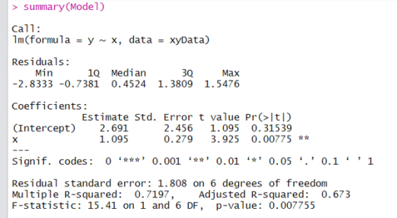
Regression Model Equation:

y =2.691 + 1.095 x .......(1)

b) Is this model useful based on...

i) R2 adjusted = 0.673 ==> It is good value make the model useful.

A model with a larger R-squared adjusted value means that the independent variables explain a larger percentage of the variation in the independent variable

ii) Hypothesis test for model coefficient

Ho: Slope of coefficient equal to Zero

H1: Slope of coefficient NOT equal to Zero

Since p-value of slope coefficient = 0.00775 which is less than 0.05 ( Alpha , level of significance)

Reject Ho

Conclusion : Independent variable 'x' is significantly predicting 'y'

iii) and iv) overall model adequacy test and regression assumptions

We will study following diagnostic plots from R output:

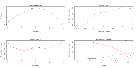
Linear Assumptions violated ( refer Residual vs Fitted plot )

Explanation: This plot shows if residuals have non-linear patterns. There could be a non-linear relationship between predictor variables and an outcome variable and the pattern could show up in this plot if the model doesn’t capture the non-linear relationship. If you find equally spread residuals around a horizontal line without distinct patterns, that is a good indication you don’t have non-linear relationships.

Normality Assumptions not violated ( refer Normal Q-Q plot )

Explanation: This plot shows if residuals are normally distributed. Do residuals follow a straight line well or do they deviate severely? It’s good if residuals are lined well on the straight dashed line.

Homoscedasticity Assumptions violated ( refer Scale-location plot )

Explanation: It’s also called Spread-Location plot. This plot shows if residuals are spread equally along the ranges of predictors. This is how you can check the assumption of equal variance (homoscedasticity). It’s good if you see a horizontal line with equally (randomly) spread points.

Influence cases and outliers Assumptions violated ( refer Residual vs Leverage plot)

Explanation: This plot helps us to find influential cases (i.e., subjects) if any. Not all outliers are influential in linear regression analysis (whatever outliers mean). Even though data have extreme values, they might not be influential to determine a regression line. That means, the results wouldn’t be much different if we either include or exclude them from analysis. They follow the trend in the majority of cases and they don’t really matter; they are not influential. On the other hand, some cases could be very influential even if they look to be within a reasonable range of the values. They could be extreme cases against a regression line and can alter the results if we exclude them from analysis.

## End of Answers ###