Compute Regression Analysis for following relationship: The relationship between death rate X1 (USD) vs. population density...
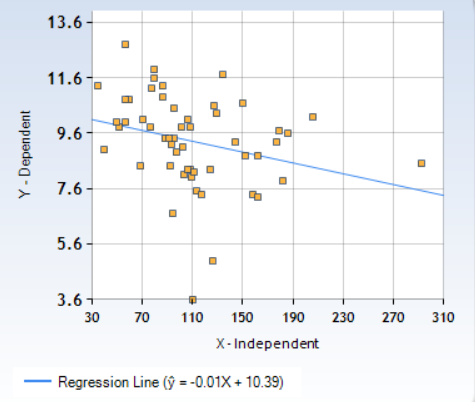
Compute Regression Analysis for following relationship: The relationship between death rate X1 (USD) vs. population density X5. Population as a Predictor, X, then death rate as a Response variable, Y. Get Regression Output, and Scatter plot between these variables and compute Coefficient of Determination, R2, and Interpret your findings.
X1 X2 X3 X4
X5 The data (X1, X2, X3, X4, X5) are by
city.
8 78 284 9.1
109 X1 = death rate per 1000 residents
9.3 68 433 8.7 144
X2 = doctor availability per 100,000 residents
7.5 70 739 7.2
113 X3 = hospital availability per 100,000
residents
8.9 96 1792 8.9
97 X4 = annual per capita income in thousands of
dollars
10.2 74 477 8.3
206 X5 = population density people per square
mile
8.3 111 362 10.9
124
8.8 77 671 10
152
8.8 168 636 9.1
162
10.7 82 329 8.7
150
11.7 89 634 7.6
134
8.5 149 631 10.8
292
8.3 60 257 9.5
108
8.2 96 284 8.8
111
7.9 83 603 9.5
182
10.3 130 686 8.7
129
7.4 145 345 11.2
158
9.6 112 1357 9.7
186
9.3 131 544 9.6
177
10.6 80 205 9.1
127
9.7 130 1264 9.2
179
11.6 140 688 8.3
80
8.1 154 354 8.4
103
9.8 118 1632 9.4
101
7.4 94 348 9.8
117
9.4 119 370 10.4
88
11.2 153 648 9.9
78
9.1 116 366 9.2
102
10.5 97 540 10.3
95
11.9 176 680 8.9
80
8.4 75 345 9.6
92
5 134 525 10.3
126
9.8 161 870 10.4
108
9.8 111 669 9.7
77
10.8 114 452 9.6
60
10.1 142 430 10.7
71
10.9 238 822 10.3
86
9.2 78 190 10.7
93
8.3 196 867 9.6
106
7.3 125 969 10.5
162
9.4 82 499 7.7
95
9.4 125 925 10.2
91
9.8 129 353 9.9
52
3.6 84 288 8.4
110
8.4 183 718 10.4
69
10.8 119 540 9.2
57
10.1 180 668 13
106
9 82 347 8.8
40
10 71 345 9.2
50
11.3 118 463 7.8
35
11.3 121 728 8.2
86
12.8 68 383 7.4
57
10 112 316 10.4
57
6.7 109 388 8.9
94
Homework Answers
| X - Mx | Y - My | (X - Mx)2 | (X - Mx)(Y - My) |
| -1.6415 | -1.3057 | 2.6946 | 2.1433 |
| 33.3585 | -0.0057 | 1112.7889 | -0.1888 |
| 2.3585 | -1.8057 | 5.5625 | -4.2586 |
| -13.6415 | -0.4057 | 186.0908 | 5.5338 |
| 95.3585 | 0.8943 | 9093.2417 | 85.2829 |
| 13.3585 | -1.0057 | 178.4493 | -13.4341 |
| 41.3585 | -0.5057 | 1710.5247 | -20.9133 |
| 51.3585 | -0.5057 | 2637.6946 | -25.97 |
| 39.3585 | 1.3943 | 1549.0908 | 54.8791 |
| 23.3585 | 2.3943 | 545.6191 | 55.9282 |
| 181.3585 | -0.8057 | 32890.9021 | -146.1133 |
| -2.6415 | -1.0057 | 6.9776 | 2.6565 |
| 0.3585 | -1.1057 | 0.1285 | -0.3964 |
| 71.3585 | -1.4057 | 5092.0342 | -100.3058 |
| 18.3585 | 0.9943 | 337.0342 | 18.2546 |
| 47.3585 | -1.9057 | 2242.8266 | -90.2492 |
| 75.3585 | 0.2943 | 5678.9021 | 22.181 |
| 66.3585 | -0.0057 | 4403.4493 | -0.3756 |
| 16.3585 | 1.2943 | 267.6002 | 21.1734 |
| 68.3585 | 0.3943 | 4672.8832 | 26.9565 |
| -30.6415 | 2.2943 | 938.9021 | -70.302 |
| -7.6415 | -1.2057 | 58.3927 | 9.2131 |
| -9.6415 | 0.4943 | 92.9587 | -4.7662 |
| 6.3585 | -1.9057 | 40.4304 | -12.1171 |
| -22.6415 | 0.0943 | 512.6379 | -2.136 |
| -32.6415 | 1.8943 | 1065.4681 | -61.8341 |
| -8.6415 | -0.2057 | 74.6757 | 1.7772 |
| -15.6415 | 1.1943 | 244.6568 | -18.6813 |
| -30.6415 | 2.5943 | 938.9021 | -79.4945 |
| -18.6415 | -0.9057 | 347.5059 | 16.8829 |
| 15.3585 | -4.3057 | 235.8832 | -66.1284 |
| -2.6415 | 0.4943 | 6.9776 | -1.3058 |
| -33.6415 | 0.4943 | 1131.7512 | -16.6303 |
| -50.6415 | 1.4943 | 2564.5625 | -75.6756 |
| -39.6415 | 0.7943 | 1571.4493 | -31.4888 |
| -24.6415 | 1.5943 | 607.204 | -39.2869 |
| -17.6415 | -0.1057 | 311.2229 | 1.864 |
| -4.6415 | -1.0057 | 21.5436 | 4.6678 |
| 51.3585 | -2.0057 | 2637.6946 | -103.0077 |
| -15.6415 | 0.0943 | 244.6568 | -1.4756 |
| -19.6415 | 0.0943 | 385.7889 | -1.853 |
| -58.6415 | 0.4943 | 3438.8266 | -28.9888 |
| -0.6415 | -5.7057 | 0.4115 | 3.6602 |
| -41.6415 | -0.9057 | 1734.0153 | 37.7131 |
| -53.6415 | 1.4943 | 2877.4115 | -80.1586 |
| -4.6415 | 0.7943 | 21.5436 | -3.6869 |
| -70.6415 | -0.3057 | 4990.2229 | 21.5923 |
| -60.6415 | 0.6943 | 3677.3927 | -42.1058 |
| -75.6415 | 1.9943 | 5721.6379 | -150.8549 |
| -24.6415 | 1.9943 | 607.204 | -49.1435 |
| -53.6415 | 3.4943 | 2877.4115 | -187.4417 |
| -53.6415 | 0.6943 | 2877.4115 | -37.2454 |
| -16.6415 | -2.6057 | 276.9398 | 43.3621 |
| SS: 115748.1887 | SP: -1132.2925 |
Sum of X = 5864
Sum of Y = 493.2
Mean X = 110.6415
Mean Y = 9.3057
Sum of squares (SSX) = 115748.1887
Sum of products (SP) = -1132.2925
Regression Equation = ŷ = bX + a
b = SP/SSX =
-1132.29/115748.19 = -0.00978
a = MY - bMX = 9.31 -
(-0.01*110.64) = 10.388
ŷ = -0.00978X + 10.388
X Values
∑ = 5864
Mean = 110.642
∑(X - Mx)2 = SSx =
115748.189
Y Values
∑ = 493.2
Mean = 9.306
∑(Y - My)2 = SSy = 143.728
X and Y Combined
N = 53
∑(X - Mx)(Y - My) = -1132.292
R Calculation
r = ∑((X - My)(Y - Mx)) /
√((SSx)(SSy))
r = -1132.292 / √((115748.189)(143.728))
r = -0.2776
The value of R is -0.2776
The value of R2, the coefficient of determination, is 0.0771
Output from excel
| SUMMARY OUTPUT | ||||||||
| Regression Statistics | ||||||||
| Multiple R | 0.277606968 | |||||||
| R Square | 0.077065629 | |||||||
| Adjusted R Square | 0.058968877 | |||||||
| Standard Error | 1.612766408 | |||||||
| Observations | 53 | |||||||
| ANOVA | ||||||||
| df | SS | MS | F | Significance F | ||||
| Regression | 1 | 11.07651198 | 11.07651198 | 4.25853365 | 0.044160289 | |||
| Residual | 51 | 132.6517899 | 2.601015488 | |||||
| Total | 52 | 143.7283019 | ||||||
| Coefficients | Standard Error | t Stat | P-value | Lower 95% | Upper 95% | Lower 95.0% | Upper 95.0% | |
| Intercept | 10.38799737 | 0.569350071 | 18.24536063 | 5.2651E-24 | 9.24497943 | 11.5310153 | 9.24497943 | 11.5310153 |
| x | -0.009782377 | 0.004740393 | -2.063621489 | 0.044160289 | -0.019299114 | -0.000265641 | -0.019299114 | -0.000265641 |
Although technically a negative correlation, the relationship between your variables is only weak (nb. the nearer the value is to zero, the weaker the relationship)
If population density people per square mile increases then death rate per 1000 residents decreases( decrease rate = 1%)
Add Answer to:
Compute Regression Analysis for following relationship: The
relationship between death rate X1 (USD) vs. population density...
Compute the correlation coefficient, r, for all five variables (columns). Interpret your findings whether you have determined any relationship between variables. X1 X2 X3 X4 X5 The data (X1, X...
Compute the correlation coefficient, r, for all five variables (columns). Interpret your findings whether you have determined any relationship between variables. X1 X2 X3 X4 X5 The data (X1, X2, X3, X4, X5) are by city. 8 78 284 9.1 109 X1 = death rate per 1000 residents 9.3 68 433 8.7 144 X2 = doctor availability per 100,000 residents 7.5 70 739 7.2 113 X3 = hospital availability per 100,000 residents 8.9 96 1792 8.9 97 X4 = annual...
Compute Regression Analysis for following relationship: The relationship between death rate X1 vs. doctor availability X2. Doctor availability as a Predictor X, then death rate as a Response variable...
Compute Regression Analysis for following relationship: The relationship between death rate X1 vs. doctor availability X2. Doctor availability as a Predictor X, then death rate as a Response variable Y. Get the Regression Output and scatter plot between the variables using data analysis toolpak in Excel. X1= Death rate per 1000 residents. X2= doctor availability per 100,000 residents. X1 X2 8 78 9.3 68 7.5 70 8.9 96 10.2 74 8.3 111 8.8 77 8.8 168 10.7 82 11.7 89...
Ms. Blankenship’s tenth grade class is studying the impact of photoperiod on plant growth. Her students...
Ms. Blankenship’s tenth grade class is studying the impact of photoperiod on plant growth. Her students fill 100 paper cups with potting soil and a single pea seed. Each cup is randomly assigned to one of four growth chambers. Each of the four growth chambers has an identical artificial light source (25 watts) but each has a different light (L) : dark cycle (D). Chamber 1 is set to 24L : 0D. Chamber 2 is set to 16L : 8D....
#2 Consider the followi ng sample of 44 observations: 8.9: 12.4: 8.6: 11.3; 9.2; 8.8;8.8; 6.2;...
 #2
Consider the followi ng sample of 44 observations: 8.9: 12.4: 8.6: 11.3; 9.2; 8.8;8.8; 6.2; .07; 7.1; 8; 10.7; 7.6; 9.1; 9.2; 8.2; 9.0; 8.7; 9.1; 10.9;10.3; 9.6; 7.8; 11.5; 9.3; 7.9; 8.8; 12.7; 8.4; 7.8; 5.7; 10.5; 10.5; 9.6; 8.9;10.2; 10.3; 7.7; 10.6; 8.3; 8.8; 9.5; 8.8; 9.4. 1. Find the mean and the standard deviation for the data given. We were unable to transcribe this image
#2
Consider the followi ng sample of 44 observations: 8.9: 12.4: 8.6: 11.3; 9.2; 8.8;8.8; 6.2; .07; 7.1; 8; 10.7; 7.6; 9.1; 9.2; 8.2; 9.0; 8.7; 9.1; 10.9;10.3; 9.6; 7.8; 11.5; 9.3; 7.9; 8.8; 12.7; 8.4; 7.8; 5.7; 10.5; 10.5; 9.6; 8.9;10.2; 10.3; 7.7; 10.6; 8.3; 8.8; 9.5; 8.8; 9.4. 1. Find the mean and the standard deviation for the data given. We were unable to transcribe this image
The following data represent soil water content (percentage of water by volume) for independent random samples...
The following data represent soil water content (percentage of water by volume) for independent random samples of soil taken from two experimental fields growing bell peppers. Soil water content from field I: x1; n1 = 72 15.2 11.3 10.1 10.8 16.6 8.3 9.1 12.3 9.1 14.3 10.7 16.1 10.2 15.2 8.9 9.5 9.6 11.3 14.0 11.3 15.6 11.2 13.8 9.0 8.4 8.2 12.0 13.9 11.6 16.0 9.6 11.4 8.4 8.0 14.1 10.9 13.2 13.8 14.6 10.2 11.5 13.1 14.7 12.5...
A particular talent competition has five judges, each of whom awards a score between 0 and...
A particular talent competition has five judges, each of whom awards a score between 0 and 10 to each performer. Fractional scores, such as 8.3, are allowed. A performer’s final score is determined by dropping the highest and the lowest score received then averaging the three remaining scores. Write a program that does the following: 1. Reads names and scores from an input file into a dynamically allocated array of structures. The first number in the input file represents the...
The data on the below shows the number of hours a particular drug is in the...
The data on the below shows the number of hours a particular drug is in the system of 200 females. Develop a histogram of this data according to the following intervals: Follow the directions. Test the hypothesis that these data are distributed exponentially. Determine the test statistic. Round to two decimal places. (sort the data first) [0, 3) [3, 6) [6, 9) [9, 12) [12, 18) [18, 24) [24, infinity) 34.7 11.8 10 7.8 2.8 20 9.8 20.4 1.2 7.2...
The data contained in the file named StateUnemp show the unemployment rate in March 2011 and...
The data contained in the file named StateUnemp show the unemployment rate in March 2011 and the unemployment rate in March 2012 for every state.† State Unemploy- ment Rate March 2011 Unemploy- ment Rate March 2012 Alabama 9.3 7.3 Alaska 7.6 7.0 Arizona 9.6 8.6 Arkansas 8.0 7.4 California 11.9 11.0 Colorado 8.5 7.8 Connecticut 9.1 7.7 Delaware 7.3 6.9 Florida 10.7 ...
An object of weight 1 N is falling vertically. The time vs. speed data can be...
An object of weight 1 N is falling vertically. The time vs. speed data can be found here. In this case the effect of air-drag cannot be neglected. Use your critical thinking to estimate the air-drag coefficient . Make sure you include the units in your answer. 0 0 0.1 0.9992 0.2 1.993 0.3 2.978 0.4 3.948 0.5 4.898 0.6 5.826 0.7 6.728 0.8 7.599 0.9 8.438 1 9.242 1.1 10.01 1.2 10.74 1.3 11.43 1.4 12.09 1.5 12.7 1.6 ...
It is commonly believed that cities with wind speeds of 10 or more have different average...
It is commonly believed that cities with wind speeds of 10 or more have different average temperature from the cities with winds of less than 10 (mp/h). Use Pollutiondata and your statistical expertise to answer the questions: Is this a reasonable belief? 4. What test/procedure did you perform? a. One-sided t-test b. Two-sided t-test c. Regression d. Confidence interval 5. Statistical Interpretation a. Since P-value is small we are confident that the slope is not zero. b. Since P-value is...
 #2
Consider the followi ng sample of 44 observations: 8.9: 12.4: 8.6: 11.3; 9.2; 8.8;8.8; 6.2; .07; 7.1; 8; 10.7; 7.6; 9.1; 9.2; 8.2; 9.0; 8.7; 9.1; 10.9;10.3; 9.6; 7.8; 11.5; 9.3; 7.9; 8.8; 12.7; 8.4; 7.8; 5.7; 10.5; 10.5; 9.6; 8.9;10.2; 10.3; 7.7; 10.6; 8.3; 8.8; 9.5; 8.8; 9.4. 1. Find the mean and the standard deviation for the data given. We were unable to transcribe this image
#2
Consider the followi ng sample of 44 observations: 8.9: 12.4: 8.6: 11.3; 9.2; 8.8;8.8; 6.2; .07; 7.1; 8; 10.7; 7.6; 9.1; 9.2; 8.2; 9.0; 8.7; 9.1; 10.9;10.3; 9.6; 7.8; 11.5; 9.3; 7.9; 8.8; 12.7; 8.4; 7.8; 5.7; 10.5; 10.5; 9.6; 8.9;10.2; 10.3; 7.7; 10.6; 8.3; 8.8; 9.5; 8.8; 9.4. 1. Find the mean and the standard deviation for the data given. We were unable to transcribe this image
Most questions answered within 3 hours.
-
For Bergson the concept of Being contains less reality than does
the concept of Becoming. True...
asked 59 minutes ago -
What is the hydroxide ion concentration, [OH-], in a solution
with a hydronium ion concentration, [H3O+]...
asked 45 minutes ago -
What species is the reducing agent in the following
equation?
Mg(s) + 2HCl (aq) --> MgCl2(aq)...
asked 1 hour ago -
A 50g ice cube is taken out of a freezer at 0 degrees Celsius
and put...
asked 2 hours ago -
How do ratios help you determine trends? What specific
information do managers look at? Is there...
asked 2 hours ago -
A wavelength of 514 nm is used to find an unknown diffraction
grating. If the separation...
asked 2 hours ago -
Use the central limit theorem to find the mean and standard
error of the mean of...
asked 3 hours ago -
You will be given a file that will contain averages for classes
which are divided into...
asked 3 hours ago -
A Pew Research Center poll surveyed a random sample 850 voters
and asked them if they...
asked 3 hours ago -
Design a class named
NumDays, to
store a value that represents a number of hours and...
asked 3 hours ago -
(R)-2-chloro-(S)-3-bromobutane and
(S)-2-chloro-(S)-3-bromobutane are: A. enantiomers. B.
diastereomers. C. meso compounds. D. the same molecule.
asked 3 hours ago -
1_ What is the Frank-Starling law of the heart? And why the
heart cannot function on...
asked 3 hours ago