Question

The data on the below shows the number of hours a particular drug is in the system of 200 females. Develop a histogram of this data according to the following intervals: Follow the directions. Test the hypothesis that these data are distributed exponentially. Determine the test statistic. Round to two decimal places.

(sort the data first)

[0, 3)

[3, 6)

[6, 9)

[9, 12)

[12, 18)

[18, 24)

[24, infinity)

34.7
11.8
10
7.8
2.8
20
9.8
20.4
1.2
7.2
23
1.7
2.4
10.3
18
4.9
1.5
5.6
25.5
20.2
8.3
3.1
6.5
0.5
3
23.8
20.6
2.1
11.7
6.8
6.6
14.5
28.2
3.4
13.5
2.5
8.5
21
1.4
9.6
12.8
29.4
0.9
1.8
35.9
9.3
7.5
19.6
33.6
20
0.7
1.6
9.4
8.8
6.4
7.9
7.3
14.2
14.4
7
27.6
25.8
4
6.2
14.6
1.2
32.6
4.2
13.4
15.3
27.9
6.6
8.8
0.8
7.6
8.9
4.7
18.8
29.7
6.2
7.2
14.3
11.5
1
11.4
19.4
8.9
22
2.2
4.5
28.8
8.7
9.5
6
8.4
3.2
24.3
32.6
4.3
2.3
18.4
0.4
27
7.4
8.6
18.2
12.1
8
19.8
8.2
10.1
7.5
7.1
3.5
16.2
10.6
10.5
5.4
3.9
1.9
24.9
8.5
19.2
3.7
25.2
6.7
5.1
13.7
18.6
3.6
30.4
10.2
3.8
3.3
6.1
2.7
14.1
0.1
5.7
0.7
1
7.9
8.3
6.9
4.6
9.1
26.4
6.3
7.4
19
16.2
14.7
28.5
6.4
8.7
5.8
7.8
27.3
8.2
7.9
6.3
29.7
0.3
6.9
8.1
8
5.3
9.9
2
0.8
4.1
7
31.5
8.1
17.9
0.2
7.1
20.8
4.4
1.1
6.5
7.6
5.9
14.6
5.2
6.7
2.6
26.1
12.5
6.8
29.1
6.1
9
9.2
15.3
10.4
11.6
30.4
35.9
6.5

Answer 1

Get the counts in the excel as below

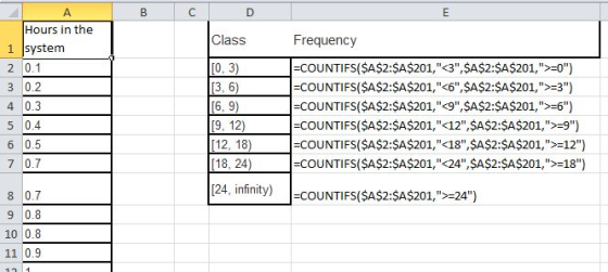
Get the follwing frequency distribution

Class	Frequency
[0, 3)	30
[3, 6)	27
[6, 9)	56
[9, 12)	21
[12, 18)	19
[18, 24)	20
[24, infinity)	27

plot the histogram using the bar graphs as below

We want to test the hypothesis that these data are distributed exponentially

Let X be the the number of hours a particular drug is in the system in females. Let X has an exponential distribution with parameter $\lambda$ and mean $\mu_x=\lambda$ and cdf is

$P(X<x)=1-e^{-\frac{x}{\lambda}}$

The sample mean is an unbiased MLE estimator of the mean of an exponential distribution. Hence the parameter can be estimated as

$\hat{\lambda} =\bar{x}=11.2765$ where $\bar{x}=\frac{\sum x}{n}=11.2765$ hours is the sample mean of the 200 observations

We want to test the hypotheses

$\begin{align*} &H_0:\text{An exponential process with } \lambda = 11.2765 \text{ is a good description of the data}\\ &H_a:\text{An exponential process with } \lambda = 11.2765 \text{ is not a good description of the data}\\ &\alpha = 0.05\leftarrow\text{level of significance to test the hypothesis} \end{align*}$

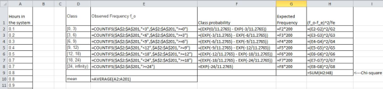
The frequency distribution gives us the observed frequency $f_o$

we need to find the frequency expected if the data were exponentially distributed.

First we find the probability that X is between the each class interval.

the probability that X is between 2 intervals [a,b) is

$\begin{align*} P(a\le X<b)&=P(X<b)-P(X\le a)\\ &=(1-e^{-\frac{b}{11.2765}})-(1-e^{-\frac{b}{11.2765}})\\ &=e^{-\frac{b}{11.2765}} - e^{-\frac{a}{11.2765}} \end{align*}$

The expected frequency of the class is $f_e=P(a\le X<b)\times 200$

For example for Class [0,3) the probability is

$\begin{align*} P(a\le X<b) &=e^{-\frac{3}{11.2765}} - e^{-\frac{0}{11.2765}} &=0.2336 \end{align*}$

The expected frequency for this class is $\begin{align*} f_e=0.2336\times 200=46.7183 \end{align*}$

For the last class [24,infty) the probability is

$P(X\ge 24) =1-P(X<24)=1-(1-e^{-\frac{24}{11.2765}}) = 0.1190$

and the expected frequency for the last class is

$f_e= 0.1190\times 200=23.8074$

Finally we get the chi-square test statistics as

$\chi^2=\sum\frac{(f_o-f_e)^2}{f_e}$

All the above calculations are in the following excel table

The values are

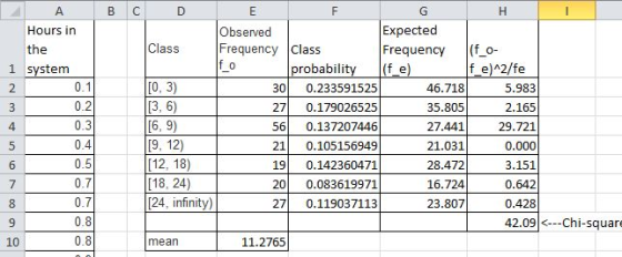
The test statistics is 42.09

Since we used the sample to estimate the parameter of exponential distribution, the degrees of freedom is k-1-1 = 7-1-1 = 5

The critical value for ch-square distribution for 0.05 level of significance is 11.070. Since the test statistics is greater than the critical value, we reject the null hypothesis.

We conclude, there is no sufficient evidence to the  the hypothesis that these data are distributed exponentially