7. Short-run supply and long-run equilibrium
![]() Screen Shot 2020-12-03 at 8.43.58 PM.png
Screen Shot 2020-12-03 at 8.43.58 PM.png
![]() Screen Shot 2020-12-03 at 8.44.19 PM.png
Screen Shot 2020-12-03 at 8.44.19 PM.png
![]() Screen Shot 2020-12-03 at 8.44.10 PM.png
Screen Shot 2020-12-03 at 8.44.10 PM.png
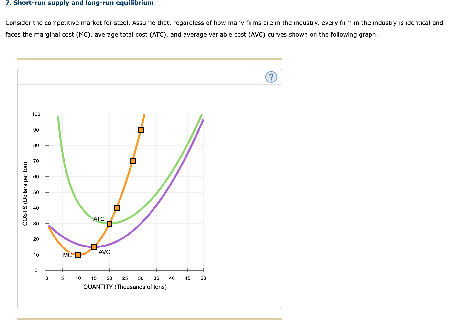
Consider the competitive market for steel. Assume that, regardless of how many firms are in the industry, every firm in the industry is identical and faces the marginal cost (MC), average total cost (ATC), and average variable cost (AVC) curves shown on the following graph.
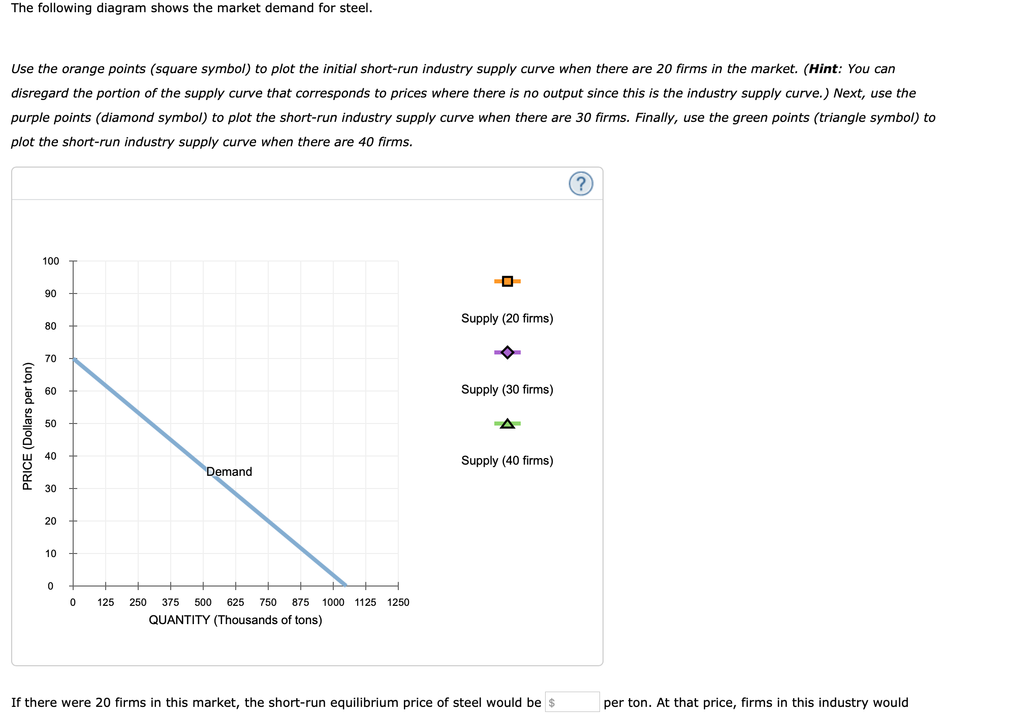
The following diagram shows the market demand for steel.
Use the orange points (square symbol) to plot the initial short-run industry supply curve when there are 20 firms in the market. (Hint: You can disregard the portion of the supply curve that corresponds to prices where there is no output since this is the industry supply curve.) Next, use the purple points (diamond symbol) to plot the short-run industry supply curve when there are 30 firms. Finally, use the green points (triangle symbol) to plot the short-run industry supply curve when there are 40 firms.
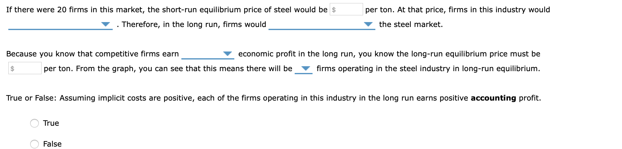
If there were 20 firms in this market, the short-run equilibrium price of steel would be . Therefore, in the long run, firms would
the steel market.
Because you know that competitive firms earn economic profit in the long run, you know the long-run equilibrium price must be
per ton. From the graph, you can see that this means there will be firms operating in the steel industry in long-run equilibrium.
True or False: Assuming implicit costs are positive, each of the firms operating in this industry in the long run earns positive accounting profit.
Homework Answers
Request Answer!
We need at least 10 more requests to produce the answer.
0 / 10 have requested this problem solution
The more requests, the faster the answer.
7. Short-run supply and long-run equilibrium Consider the competitive market for steel. Assume that, regardless of...
 7. Short-run supply and long-run equilibrium Consider the competitive market for steel. Assume that, regardless of how many firms are in the industry, every firm in the industry is identical and faces the marginal cost (MC), average total cost (ATC), and average variable cost (AVC) curves shown on the following graph. BO 72 54 ATC COSTS (Dollars per ton) 40 32 24 AVC 8 МСС 3 27 30 12 15 18 21 24 QUANTITY (Thousands of tons) The following diagram...
5. Short-run supply and long-run equilibrium Consider the perfectly competitive market for steel. Assume that, regardless...
 5. Short-run supply and long-run equilibrium Consider the perfectly competitive market for steel. Assume that, regardless of how many firms are in the industry, every firm in the industry is identical and faces the marginal cost (MC), average total cost (ATC), and average variable cost (AVC) curves shown on the following graph. COSTS (Dollars per ton) + MC D AVC 0 10 90 100 20 30 40 50 60 70 80 QUANTITY (Thousands of tons) The following diagram shows the...
7. Short-run supply and long-run equillbrium Consider the competitive market for steel. Assume that, regardless of...
 7. Short-run supply and long-run equillbrium Consider the competitive market for steel. Assume that, regardless of how many firms are in the industry, every firm in the industry is identical and faces the marginal cost (MC), average total cost (ATC), and average variable cost (AVC) curves shown on the following graph 100 90 27.5, 70 80 70 30 20 AVC 10 0s10 1520 25 30 35 40 45 QUANTITY (Thousands of tons) The following diagram shows the market demand for...
7. Short-run supply and long-run equilibrium Aa Aa Consider a perfectly competitive market for titanium. Assume...
 7. Short-run supply and long-run equilibrium Aa Aa Consider a perfectly competitive market for titanium. Assume that all firms in the industry are identical and have the marginal cost (MC), average total cost (ATC), and average variable cost (AVC) curves shown on the following graph. Assume also that it does not matter how many firms are in the industry. Tool Tip: Place the mouse cursor over orange square points on the MC curve to see coordinates. COSTS (Dollars per kilogram...
7. Short-run supply and long-run equilibrium Consider the competitive market for titanium. Assume that, regardless of...
 7. Short-run supply and long-run equilibrium Consider the competitive market for titanium. Assume that, regardless of how many firms are in the industry, every firm in the industry is identical and faces the marginal cost (MC), average total cost (ATC), and average variable cost (AVC) curves shown on the following graph. COSTS (Dollars per pound) + MC O AVC 0 5 45 50 10 15 20 25 30 35 40 QUANTITY (Thousands of pounds) The following diagram shows the market...
7. Short-run supply and long-run equilibrium Consider the competitive market for copper. Assume that, regardless of...
 7. Short-run supply and long-run
equilibrium
Consider the competitive market for copper. Assume that,
regardless of how many firms are in the industry, every firm in the
industry is identical and faces the marginal cost (MC), average
total cost (ATC), and average variable cost (AVC) curves shown on
the following graph.
The following diagram shows the market demand for copper.
Use the orange points (square symbol) to plot the initial
short-run industry supply curve when there are 10 firms in...
7. Short-run supply and long-run
equilibrium
Consider the competitive market for copper. Assume that,
regardless of how many firms are in the industry, every firm in the
industry is identical and faces the marginal cost (MC), average
total cost (ATC), and average variable cost (AVC) curves shown on
the following graph.
The following diagram shows the market demand for copper.
Use the orange points (square symbol) to plot the initial
short-run industry supply curve when there are 10 firms in...
7. Short-run supply and long-run equilibrium Consider the competitive market for copper. Assume that, regardless of...
 7. Short-run supply and long-run equilibrium Consider the competitive market for copper. Assume that, regardless of how many firms are in the industry, every firm in the industry is identical and faces the marginal cost (MC), average total cost (ATC), and average variable cost (AVC) curves shown on the following graph. COSTS (Dollars per pound) MC D AVC 0 + 0 + 10 + + + + + + + 20 30 40 50 60 70 80 QUANTITY (Thousands of...
Short-run supply and long-run equilibrium, please and thank you Consider the competitive market for titanium. Assume...
 Short-run supply and long-run equilibrium, please and
thank you
Consider the competitive market for titanium. Assume that, regardless of how many firms are in the industry, every firm in the industry is identical and faces the marginal cost (MC), average total cost (ATC), and average variable cost (AVC) curves shown on the following graph. COSTS (Dollars per kilogram) ATC + MC O AVC ott 0 5 10 15 20 25 30 35 40 QUANTITY (Thousands of kilograms) 45 50 The...
Short-run supply and long-run equilibrium, please and
thank you
Consider the competitive market for titanium. Assume that, regardless of how many firms are in the industry, every firm in the industry is identical and faces the marginal cost (MC), average total cost (ATC), and average variable cost (AVC) curves shown on the following graph. COSTS (Dollars per kilogram) ATC + MC O AVC ott 0 5 10 15 20 25 30 35 40 QUANTITY (Thousands of kilograms) 45 50 The...
7. Short-run supply and long-run equilibrium Consider the competitive market for titanium. Assume that, regardless of...
 7. Short-run supply and long-run equilibrium Consider the competitive market for titanium. Assume that, regardless of how many firms are in the industry, every firm in the industry is identi and faces the marginal cost (MC), average total cost (ATC), and average variable cost (AVC) curves shown on the following graph. COSTS (Dollars per pound) AVC мс о OFFFFF 0 3 6 9 12 15 18 21 24 QUANTITY (Thousands of pounds) 27 30 The following diagram shows the market...
7. Short-run supply and long-run equilibrium Consider the competitive market for titanium. Assume that, regardless of...
 7. Short-run supply and long-run equilibrium Consider the competitive market for titanium. Assume that, regardless of how many firms are in the industry, every firm in the industry is identical and faces the marginal cost (MC), average total cost (ATC), and average variable cost (AVC) curves shown on the following graph. 100 T 90 - 80 60 50 40 30 20 0 5 10 15 20 25 30 35 4045 50 QUANTITY (Thousands of pounds) The following diagram shows the...
 7. Short-run supply and long-run equilibrium Consider the competitive market for steel. Assume that, regardless of how many firms are in the industry, every firm in the industry is identical and faces the marginal cost (MC), average total cost (ATC), and average variable cost (AVC) curves shown on the following graph. BO 72 54 ATC COSTS (Dollars per ton) 40 32 24 AVC 8 МСС 3 27 30 12 15 18 21 24 QUANTITY (Thousands of tons) The following diagram...
 5. Short-run supply and long-run equilibrium Consider the perfectly competitive market for steel. Assume that, regardless of how many firms are in the industry, every firm in the industry is identical and faces the marginal cost (MC), average total cost (ATC), and average variable cost (AVC) curves shown on the following graph. COSTS (Dollars per ton) + MC D AVC 0 10 90 100 20 30 40 50 60 70 80 QUANTITY (Thousands of tons) The following diagram shows the...
 7. Short-run supply and long-run equillbrium Consider the competitive market for steel. Assume that, regardless of how many firms are in the industry, every firm in the industry is identical and faces the marginal cost (MC), average total cost (ATC), and average variable cost (AVC) curves shown on the following graph 100 90 27.5, 70 80 70 30 20 AVC 10 0s10 1520 25 30 35 40 45 QUANTITY (Thousands of tons) The following diagram shows the market demand for...
 7. Short-run supply and long-run equilibrium Aa Aa Consider a perfectly competitive market for titanium. Assume that all firms in the industry are identical and have the marginal cost (MC), average total cost (ATC), and average variable cost (AVC) curves shown on the following graph. Assume also that it does not matter how many firms are in the industry. Tool Tip: Place the mouse cursor over orange square points on the MC curve to see coordinates. COSTS (Dollars per kilogram...
 7. Short-run supply and long-run equilibrium Consider the competitive market for titanium. Assume that, regardless of how many firms are in the industry, every firm in the industry is identical and faces the marginal cost (MC), average total cost (ATC), and average variable cost (AVC) curves shown on the following graph. COSTS (Dollars per pound) + MC O AVC 0 5 45 50 10 15 20 25 30 35 40 QUANTITY (Thousands of pounds) The following diagram shows the market...
 7. Short-run supply and long-run
equilibrium
Consider the competitive market for copper. Assume that,
regardless of how many firms are in the industry, every firm in the
industry is identical and faces the marginal cost (MC), average
total cost (ATC), and average variable cost (AVC) curves shown on
the following graph.
The following diagram shows the market demand for copper.
Use the orange points (square symbol) to plot the initial
short-run industry supply curve when there are 10 firms in...
7. Short-run supply and long-run
equilibrium
Consider the competitive market for copper. Assume that,
regardless of how many firms are in the industry, every firm in the
industry is identical and faces the marginal cost (MC), average
total cost (ATC), and average variable cost (AVC) curves shown on
the following graph.
The following diagram shows the market demand for copper.
Use the orange points (square symbol) to plot the initial
short-run industry supply curve when there are 10 firms in...
 7. Short-run supply and long-run equilibrium Consider the competitive market for copper. Assume that, regardless of how many firms are in the industry, every firm in the industry is identical and faces the marginal cost (MC), average total cost (ATC), and average variable cost (AVC) curves shown on the following graph. COSTS (Dollars per pound) MC D AVC 0 + 0 + 10 + + + + + + + 20 30 40 50 60 70 80 QUANTITY (Thousands of...
 Short-run supply and long-run equilibrium, please and
thank you
Consider the competitive market for titanium. Assume that, regardless of how many firms are in the industry, every firm in the industry is identical and faces the marginal cost (MC), average total cost (ATC), and average variable cost (AVC) curves shown on the following graph. COSTS (Dollars per kilogram) ATC + MC O AVC ott 0 5 10 15 20 25 30 35 40 QUANTITY (Thousands of kilograms) 45 50 The...
Short-run supply and long-run equilibrium, please and
thank you
Consider the competitive market for titanium. Assume that, regardless of how many firms are in the industry, every firm in the industry is identical and faces the marginal cost (MC), average total cost (ATC), and average variable cost (AVC) curves shown on the following graph. COSTS (Dollars per kilogram) ATC + MC O AVC ott 0 5 10 15 20 25 30 35 40 QUANTITY (Thousands of kilograms) 45 50 The...
 7. Short-run supply and long-run equilibrium Consider the competitive market for titanium. Assume that, regardless of how many firms are in the industry, every firm in the industry is identi and faces the marginal cost (MC), average total cost (ATC), and average variable cost (AVC) curves shown on the following graph. COSTS (Dollars per pound) AVC мс о OFFFFF 0 3 6 9 12 15 18 21 24 QUANTITY (Thousands of pounds) 27 30 The following diagram shows the market...
 7. Short-run supply and long-run equilibrium Consider the competitive market for titanium. Assume that, regardless of how many firms are in the industry, every firm in the industry is identical and faces the marginal cost (MC), average total cost (ATC), and average variable cost (AVC) curves shown on the following graph. 100 T 90 - 80 60 50 40 30 20 0 5 10 15 20 25 30 35 4045 50 QUANTITY (Thousands of pounds) The following diagram shows the...
Most questions answered within 3 hours.
-
Buying your in-laws a gift because it’s expected is
due to the ____________ motive of gift-giving....
asked 6 minutes ago -
Discuss the pros and cons of collaborative software such
as SameTime. Does it increase productivity? What...
asked 3 minutes ago -
A large cable company reports the following.
80% of its customers subscribe to its cable TV...
asked 5 minutes ago -
Calculate the expected value, the variance, and the standard
deviation of the given random variable X....
asked 49 minutes ago -
A hospital performs 100 surgeries per week. The probability that
complications after surgery occur is 10%....
asked 1 hour ago -
1 point) Given the significance level α=0.01 find the following:
(a) left-tailed z value z= (b)...
asked 47 minutes ago -
Assuming you are the head of the software development unit at
Cyber.Soft, explain and justify why...
asked 14 minutes ago -
Magnesium and nitrogen react in a combination reaction to
produce magnesium nitride. 3 Mg + N2...
asked 22 minutes ago -
Two electrons are initially at rest separated by a distance of
2nm. At time t=0, they...
asked 19 minutes ago -
A martial artist is practicing breaking 5 boards. He is able to
break aboard with probability...
asked 27 minutes ago -
The rate constant of a first-order reaction is 2.95 × 10⁻⁴ s−1
at 350.° C. If...
asked 30 minutes ago -
implement a class called PiggyBank that will be used to
represent a collection of coins. Functionality...
asked 21 minutes ago