Question

Could anyone help me with the lookup function for #5?

Plain Text Tahoma Start Excel. Open the file named ex02TravelAgency START Save the file with the name 0.000 ex02TravelAgency LastFirst, replacing LastFirst with your name. On the Agency Clients worksheet, apply the Table Style Light 14 to the Clients named range. Note, the style may be named Green, Table Style Light 14, depending on the version of Office used. 2 2.000 3 named ranges for each of the column headings in the Clients named range. 2.000 a named range for the range C14:E18 on the Agency Data and Analysis worksheet with the name 4 2.000 RewardLookup n the points can be found on the Agency Data and Analysis worksheet. Apply conditional formatting to the Reward Points YTD column using the Ratings 3 Stars icon set and the Agency Clients worksheet in cell K9, use a VLOOKUP function to determine the reward points earned based on total spent. Use the RewardLookup named range. The breakdown of the reward 5 8.000 6 4.000 fault settings. In cell B4, use the MAX function to calculate the maximum amount spent by the clients, using the Total_Spent named range. Format as Accounting with 2 decimal places. 2.000 In cell B5, use the AVERAGE function to calculate the average amount spent by the clients, using the Total Spent named range. Format as Accounting with 2 decimal places. 8 2.000

Answer 1

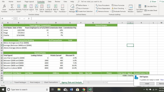
The Vlookup function is explained as follows:

Syntax

=VLOOKUP (Lookup_value, table_array, col_index_number, [range_lookup])

Arguments

		Formula items for Cell K9
Lookup_value	value to look for in the first column of a table (total spent)	I9
table_array	Table array from which to retrieve a value (lookup array in sheet Agency Data and Analysis)	Agency Data and Analysis!$C$14:$D$18
col_index_number	column in the table from which to retrieve a value. (Points Earned)	2
[range_lookup]	[optional] TRUE = approximate match (default). FALSE = exact match. Since data is given as greater than total spent will get respective rewards)	True or 1

For Cell K9: =VLOOKUP(I9, Agency Data and Analysis!$C$14:$D$18,2,1)

Copy above formula for rest of cells in I^th column to get the rewards point.