Question

1. Consider the IS-LM and aggregate demand/aggregate supply model of Chapters 11 and 12. Consider a reduction in the level of taxes, starting from an initial situation in which output is equal to its natural level.
   

a) Depict the short-run effects of the reduction in T using 3 graphs: one for the market for goods and services, one for the IS-LM curves, and one for the Aggregate Demand and Supply curves. How do the new short-run equilibrium values of r, Y and P compare to the initial ones? (i.e., are they higher, lower or equal?)

b) Depict the transition from the short-run to the long run. To do this, draw 3 new graphs (with the same variables as before), in which the initial situation is the short-run equilibrium after the decrease in T. How do the long-run equilibrium values of r, Y and P after the shock in T compare to ones before that shock?

Note: be sure to label: i. the axes; ii. the curves; iii. the initial equilibrium values; iv. the direction the curves shift (including the initial adverse shock); and v. the terminal equilibrium values.

Answer 1

(a)

(1) Goods market

Lower tax will increase consumption and decrease savings. Savings function shifts left, increasing interest rate and decreasing savings/investment in short run.

In following graph, S0 and I0 are initial saving & investment curves intersecting at point A with initial interest rate r0 and saving/investment Q0. When tax falls in short run, S0 shifts left to S1, intersecting I0 at point B with higher interest rate r1 and lower savings/investment Q1.

SO

(2) IS-LM

Lower tax will increase consumption, shifting IS curve rightward, increasing interest rate and output in short run.

In following graph, IS0 and LM0 are initial IS & LM curves intersecting at point A with initial interest rate r0 and output Y0. When tax falls in short run, IS0 shifts right to IS1, intersecting LM0 at point B with higher interest rate r1 and higher output Y1.

- LMO N 150 Yo Y

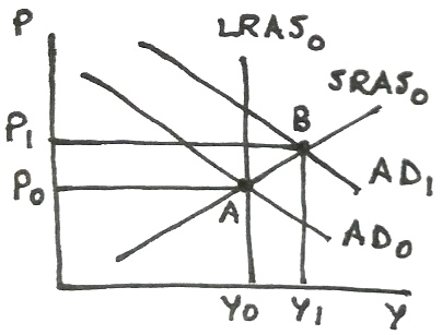
(3) AD-AS

Increase in consumption will increasing aggregate demand, shifting AD curve rightward, increasing price level and real GDP in short run.

In following graph, AD0, LRAS0 and SRAS0 are initial aggregate demand, long-run aggregate supply and short-run aggregate supply curves intersecting at point A with initial price level P0 and real GDP (potential GDP) Y0. Higher consumption shifts AD0 rightward, intersecting SRAS0 at point B with higher price level P1 and higher real GDP Y1 in short run.

LRAS E XAD, \AD, HADO Yo Y Y

(b)

(1) Goods market

In long run, higher interest rate decreases investment. Investment function shifts left, decreasing interest rate until it falls to initial level, and further decreasing savings/investment.

In following graph, I0 shifts left to I1, intersecting S1 at point B with initial interest rate r0 and further lower savings/investment Q2.

مکہ وو او 92

(2) IS LM

In long run, higher interest rate decreases demand for money, which shifts LM curve rightward, decreasing interest rate until it falls to initial level, and further increasing real GDP.

In following graph, LM0 shifts right to LM1, intersecting IS1 at point C with initial interest rate r0 and further higher output Y2.

y ۷۰ ۷۱ ۷2 owe sil "sil |

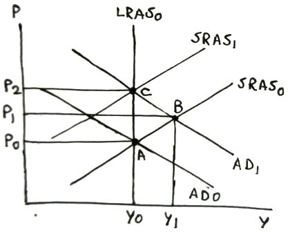
(3) AD AS

In the long run, higher price level will increase prices of inputs. Firms will reduce output, decreasing aggregate supply. SRAS shifts leftward, intersecting new AD curve at further higher price level and real GDP being restored to the potential GDP.

In following graph, in long run, SRAS0 shifts left to SRAS1, intersecting AD1 at point C with further higher price level P2 and restoring real GDP to potential GDP level Y0.

LRASO SRAS SRASO ADO H YO Y