Question

4) Consider the stable second-order continuous transfer function (in s domain): H = S +1 S2 + 3s + 2 Using the command Hd = c2d (H, Ts) with Ts = 0.1, convert H to the z domain. On the same Figure, plot the continuous impulse response of the system against the discrete one. Considering your work in problem 4, 5) Vary Ts (Ts = 0.7, 0.5, 0.3, 0.1) and observe the plot of the continuous impulse response of the system against the discrete one. What is the relationship between Ts and the precision of the approximation? 6) What disadvantage a very large Ts might cause? What disadvantage a very small Ts might produce?

Using MATLAB

Answer 1

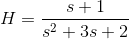
Q4) For the given question, the transfer function is :

$H = \frac{s+1}{s^{2}+3s+2}$

So first we write a MATLAB code to create this transfer function and to convert it to the z domain for the given sampling time Ts = 0.1s. The code snippet to do the same is as follows:

clear
clc
close all

% create a polynomial vector that represents the numerator 
% and the denominator of the polynomial
num = [1 1];
den = [1 3 2];

% the numerator and denominator are put together to get 
% transfer function
H = tf(num,den)

% sampling time is considered as 0.1s
Ts = 0.1;
% continuous domain in s is converted into discrete domain in z
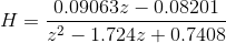
Hd = c2d(H,Ts)

The output of this section of code can be seen as the transfer functions being displayed on the command window of MATLAB:

\

Command Window H = s + 1 s^2 + 3 s + 2 Continuous-time transfer function. Hd = 0.09063 z - 0.08201 Z^2 - 1.724 z + 0.7408 Sample time: 0.1 seconds Discrete-time transfer function.

The z domain transfer function obtained is as follows (as in the above image):

H 0.090632 0.08201 22 – 1.724z +0.7408

The impulse response of the two transfer functions can be plotted on the same figure in MATLAB using the following piece of code:

% impulse response of the original transfer function 
% for a time of 3s
impulse(H,3)
hold on      % command to make the next plot on the same figure 
% impulse response of discrete time transfer function
impulse(Hd,'r') 
legend('continuous time','Ts = 0.1')

The impulse response of obtained is as follows:

Impulse Response 1 0.9 continuous time Ts = 0.1 0.8 0.7 0.6 Amplitude 0.5 0.4 0.3 0.2 0.1 0 0 0.5 1 2 2.5 الم 1.5 Time (seconds)

Here, we can see that the discrete domain impulse response behaves similar to the continuous domain impulse response and is a form of approximation of the continuous one. Thus, there is an error between the two.

Q5) Now, in the previous question we vary the sampling times and see the changes in the plots. We consider the sampling times as Ts = {0.1,0.3,0.5,0.7}.

The entire code for this is as follows:

clear
clc
close all

% create a polynomial vector that represents the numerator 
% and the denominator of the polynomial
num = [1 1];
den = [1 3 2];

% the numerator and denominator are put together to get 
% transfer function
H = tf(num,den)

% sampling time is considered as 0.1s
Ts = 0.1;
% continuous domain in s is converted into discrete domain in z
Hd = c2d(H,Ts)

% impulse response of the original transfer function 
% for a time of 3s
impulse(H,3)
hold on      % command to make the next plot on the same figure 
% impulse response of discrete time transfer function
impulse(Hd,'r') 

% plot for 0.3s sampling time
Ts = 0.3;
Hd = c2d(H,Ts)
impulse(Hd,'g')

% plot for 0.5s sampling time
Ts = 0.5;
Hd = c2d(H,Ts)
impulse(Hd,'m')

% plot for 0.7s sampling time
Ts = 0.7;
Hd = c2d(H,Ts)
impulse(Hd,'c')
legend('continuous time','Ts = 0.1','Ts = 0.3','Ts = 0.5','Ts = 0.7')

The output plot we obtain from this is as follows:

Impulse Response 1 0.9 continuous time Ts = 0.1 Ts = 0.3 Ts = 0.5 Ts = 0.7 0.8 0.7 0.6 Amplitude 0.5 0.4 0.3 0.2 0.1 0 0 0.5 1 2 2.5 3 1.5 Time (seconds)

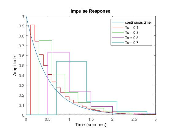
As can be remarked from the figure, the precision of the approximations of the impulse response obtained from discrete domain transfer functions decreases progressively as the sampling time Ts increases. The red one closely tracks the original blue one while the error is greater in the green which is largest in the one represented by cyan.

Thus, we can conclude that smaller the sampling time better the precision of the approximation.

Q6) A very large Ts as seen in the above solution can cause a great lack of precision and be far off from the original one. While the issue with a very small Ts is that the computational load on the device is increased. Thus, a tradeoff between precision and computational cost needs to be achieved. For example, a Ts = 0.01 produces a pretty precise plot as shown below:

Impulse Response 1 0.9 0.8 0.7 0. 6 Amplitude 0.5 0.4 0.3 0.2 0.1 0 0 0.5 1 2.5 تی N 1.5 Time (seconds)

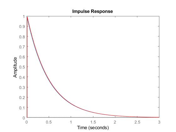
Here we can see that the two plots almost coincide with only a marginal error. Thus, depending on the device performing this operation, we need to decide the sampling time. For example, if this operation is to be performed in a low-level digital controller, then the sampling time might be decided by some other circuit parameters and even if left on the designer's discretion, taking a very small value might be too tasking for the controller. While if the same is to be performed on a computer, it might be trivial and even smaller Ts values can be taken.