Question

In this exercise use the Peruvian blood pressure data set, provided in the file peruvian.txt. This dataset consists of variables possibly relating to blood pressures of n = 39 Peruvians who have moved from rural high altitude areas to urban lower altitude areas. The variables in this dataset are: Age, Years, Weight, Height, Calf, Pulse, Systol and Diastol. Before reading the data intoMATLAB, it can be viewed in a text editor.

This question involves the use of multiple linear regression on the Peru data set.

a) Use the fitlm() function to perform a multiple linear regression with Systol as the response and the other variables as predictors. Comment on the output. For example:

Is there a relationship between the predictors and the response? 

Which predictors appear to have a statistically significant relationship to the

response? 

What does the coefficient for the Weight variable suggest? 


Use the plotResiduals() and PlotDiagnostics function to produce diagnostic plots of the least squares regression fit. Comment on any problems you see with the fit.

b) Fit a with

Is there a relationship between the predictors and the response? 

Which predictors appear to have a statistically significant relationship to the

response? 

What does the coefficient for the Weight variable suggest? 


Use the plotResiduals() and PlotDiagnostics function to produce diagnostic plots of the least squares regression fit. Comment on any problems you see with the fit.

smaller model that only uses the predictors for which there is evidence of association the response. How well do the models in (a) and (b) fit the data?

c) Use the * symbol to fit linear regression models with interaction effects. Do any interactions appear to be statistically significant? Compare the model to the models in (a) and (b). 


d) Using the information from the correlation matrix you computed above, develop a rational approach to fit a model. Which predictors have you picked and why? How well does the model fit the data? Compare this model to the previous models.

Analysis of Variance Source Regression 9 4358.85 484.32 Error Total DF Adj SS Adj MS F-Value P-Value 6.46 0.000 29 2172.58 74.92 38 6531.44 Model Summary R-sq 8.65544 66.748 S R-Sq (adj) 56.418 R-sq (pred) 34 . 45% Coefficients Term Coef SE Coef T-Value P-Value VIF 49.0 0.815 0.431 3.00 0.006 Constant146.8 Age Years 1.121 0.327 -3.43 0.002 3.21 2.455 FracLife -115.3 0.005 34.29 30.2 -3.82 0.001 24.39 3.01 3.28 0.003 4.75 Height -0.0346 0.0369 -0.94 0.355 1.91 -0.944 0.741 -1.270.213 2.06 1.19 -0.98 0.335 3.80 -0.159 0.537 -0.30 0.770 2.41 0.67 0.507 1.33 Weight 1.414 Chin Forearm Calf Pulse 0.115 0.170

Answer 1

This dataset consists of variables possibly relating to blood pressures of n = 39 Peruvians who have moved from rural high altitude areas to urban lower altitude areas (peru.txt). The variables in this dataset are:

Y = systolic blood pressure
X₁ = age
X₂ = years in urban area
X₃ = X₂ /X₁ = fraction of life in urban area
X₄ = weight (kg)
X₅ = height (mm)
X₆ = chin skinfold
X₇ = forearm skinfold
X₈ = calf skinfold
X₉ = resting pulse rate

First, we run a multiple regression using all nine x-variables as predictors. The results are given below.

Analysis of Variance Source Regression 9 4358.85 484.32 Error Total DF Adj SS Adj MS F-Value P-Value 6.46 0.000 29 2172.58 74.92 38 6531.44 Model Summary R-sq 8.65544 66.748 S R-Sq (adj) 56.418 R-sq (pred) 34 . 45% Coefficients Term Coef SE Coef T-Value P-Value VIF 49.0 0.815 0.431 3.00 0.006 Constant146.8 Age Years 1.121 0.327 -3.43 0.002 3.21 2.455 FracLife -115.3 0.005 34.29 30.2 -3.82 0.001 24.39 3.01 3.28 0.003 4.75 Height -0.0346 0.0369 -0.94 0.355 1.91 -0.944 0.741 -1.270.213 2.06 1.19 -0.98 0.335 3.80 -0.159 0.537 -0.30 0.770 2.41 0.67 0.507 1.33 Weight 1.414 Chin Forearm Calf Pulse 0.115 0.170

When looking at tests for individual variables, we see that p-values for the variables Height, Chin, Forearm,Calf, and Pulse are not at a statistically significant level. These individual tests are affected by correlations amongst the x-variables, so we will use the General Linear F procedure to see whether it is reasonable to declare that all five non-significant variables can be dropped from the model.

Next, consider testing:

H₀ : β₅ = β₆ = β₇ = β₈ = β₉ = 0
H_A : at least one of {β₅ , β₆ , β₇ , β₈ , β₉ } ≠ 0

within the nine variable model given above. If this null is not rejected, it is reasonable to say that none of the five variables Height, Chin, Forearm, Calf and Pulse contribute to the prediction/explanation of systolic blood pressure.

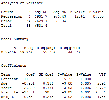
The full model includes all nine variables; SSE(full) = 2172.58, the full error df = 29, and MSE(full) = 74.92 (we get these from the Minitab results above). The reduced modelincludes only the variables Age, Years, fraclife, and Weight (which are the remaining variables if the five possibly non-significant variables are dropped). Regression results for the reduced model are given below.

Analysis of Variance Source Regression 4 3901.7 975.43 12.61 0.000 Error Total DF Adj SS Adj MS F-Value P-Value 34 2629.777.34 38 6531.4 Model Summary S R-sq R-sq (adj) R-sq (pred) 8.79456 59.74 55.00 44.84 Coefficients Term Constant Coef SE Coef T-Value P-Value VIF 116.8 2.339 0.832 5.32 0.000 Years FracLife -108.1 Weight -0.951 0.316 -3.00 0.005 2.91 3.03 0.005 29.79 28.3 -3.81 0.001 20.83 3.02 0.005 1.88 22.0 0.771 0.275

We see that SSE(reduced) = 2629.7, and the reduced error df = 34. We also see that all four individual x-variables are statistically significant.

The calculation for the general linear F-test statistic is:

F=SSE(reduced) - SSE(full)error df for reduced - error df for fullMSE(full)=2629.7−2172.5834−2974.92=1.220F=SSE(reduced) - SSE(full)error df for reduced - error df for fullMSE(full)=2629.7−2172.5834−2974.92=1.220

Thus, this test statistic comes from an F_5,29distribution, of which the associated p-value is 0.325 (this can be done by using Calc >> Probability Distribution >> F in Minitab). This is not at a statistically significant level, so we do not reject the null hypothesis. Thus it is feasible to drop the variables X₅, X₆, X₇, X₈, and X₉ from the model.

Example: Measurements of College Students

For n = 55 college students, we have measurements (Physical.txt) for the following five variables:

Y = height (in)
X₁ = left forearm length (cm)
X₂ = left foot length (cm)
X₃ = head circumference (cm)
X₄ = nose length (cm)

The Minitab output for the full model is given below.

Coefficients Term Constant 18.50 7.83 2.78, 34.23) 2.36 0.022 LeftArm 0.8020.171 0.459, 1.145) 4.70 0.000 1.63 LeftFoot 0.997 0.162 0.671, 1.323) 6.14 0.000 1.86 Headcirc 0.081 50 (0.220, 0.381) Coef SE Coef 95% CI T-Value P-Value VI 0.54 0.593 1.28 -0.1470.492 (1.136, 0.841)-0.30 0.766 1.14 noge Regression Equation Height = 18.50 + 0.802 LeftArm + 0.997 LeftFoot + 0.081 HeadCírc - 0.147 nose

Notice in the output that there are also t-test results provided. The interpretations of these t-tests are as follows:

• The sample coefficients for LeftArm and LeftFoot achieve statistical significance. This indicates that they are useful as predictors of Height.
• The sample coefficients for HeadCirc and nose are not significant. Each t-test considers the question of whether the variable is needed, given that all other variables will remain in the model.

Below is a plot of residuals versus the fitted values and it seems suitable.

Versus Fits (response is Height) an 2.5 -2.5 5.0 60 62 64 68 70 72 74 76 Fitted Value

There is no obvious curvature and the variance is reasonably constant. One may note two possible outliers, but nothing serious.

The first calculation we will perform is for the general linear F-test. The results above might lead us to test

H₀ : β₃ = β₄ = 0
H_A : at least one of {β₃ , β₄} ≠ 0

in the full model. If we fail to reject the null hypothesis, we could then remove both of HeadCirc and noseas predictors.

Below is the ANOVA table for the full model.

Analysis of Variance Source DF Seq SS Seq MS F-Value P-Value Regression 4816.39 204.098 42.81 0.000 LeftArm 590.21 590.214 123.81 0.000 LeftFoot 224.35 224.349 47.06 0.000 HeadCirc 0.29 0.590 nose 1 1.40 1.402 1 0.43 0.4270.09 0.766 Error Total 50 238.35 4.767 54 1054.75

From this output, we see that SSE(full) = 238.35, with df = 50, and MSE(full) = 4.77. The reduced model includes only the two variables LeftArm and LeftFoot as predictors. The ANOVA results for the reduced model are found below.

Analysis of Variance DF Seq SS Seq MS F-Value P-Value 2 814.56 407.28188.18 0.000 1 590.21 590.214 127.78 0.000 49 48.57 0.000 Source Regression LeftArm LeftFoot 52 240.18 Lack-of-Fit 44 175.14 3.9800.49 0.937 1 224.35 224.3 Error Pure Error 8 65.04 8.130 Total 54 1054.75

From this output, we see that SSE(reduced) = SSE(X₁ , X₂) = 240.18, with df = 52, and MSE(reduced) = MSE(X₁ , X₂) = 4.62.

With these values obtained, we can now obtain the test statistic for testing H₀ : β₃ = β₄ = 0:

F=SSE(X1,X2)−SSE(full)error df for reduced - error df for fullMSE(full)=240.18−238.3552−504.77=0.192F=SSE(X1,X2)−SSE(full)error df for reduced - error df for fullMSE(full)=240.18−238.3552−504.77=0.192

This value comes from an F_2,50 distribution. By using Calc >> Probability Distribution >> Fin Minitab, we learn that the area to the left of F = 0.192 (with df of 2 and 50) is 0.174. The p-value is the area to the right of F, so p = 1 − 0.174 = 0.826. Thus, we do not reject the null hypothesis and it is reasonable to removeHeadCirc and nose from the model.

Next we consider what fraction of variation in Y = Height cannot be explained by X₂ = LeftFoot, but can be explained by X₁ = LeftArm? To answer this question, we calculate the partial R². The formula is:

R2Y,1|2=SSR(X1|X2)SSE(X2)=SSE(X2)−SSE(X1,X2)SSE(X2)RY,1|22=SSR(X1|X2)SSE(X2)=SSE(X2)−SSE(X1,X2)SSE(X2)

The denominator, SSE(X₂), measures the unexplained variation in Y when X₂ is the predictor. The ANOVA table for this regression is found in below.

Analysis of Variance DF Seq SS Seq MS F-Value P-Value 1 707.4 707.420 107.95 0.000 1 707.4 707.420 107.95 0.000 Source Regression LeftFoot Error 53 347.3 6.553 Lack-of-Fit 19 113.0 5.948 0.86 0.625 Pure Error 34 234.3 6.892 Total 54 1054.7

These results give us SSE(X₂) = 347.3.

The numerator, SSE(X₂)–SSE(X₁,  X₂ ), measures the further reduction in the SSE when X₁ is added to the model. Results from the earlier Minitab output give us SSE(X₁,  X₂) = 240.18 and now we can calculate:

R2Y,1|2=SSR(X1|X2)SSE(X2)=SSE(X2)−SSE(X1,X2)SSE(X2)=347.3−240.18347.3=0.308RY,1|22=SSR(X1|X2)SSE(X2)=SSE(X2)−SSE(X1,X2)SSE(X2)=347.3−240.18347.3=0.308

Thus X₁ = LeftArm explains 30.8% of the variation in Y = Height that could not be explained by X₂ =LeftFoot.

‹ 6.6 - Lack of Fit