Question

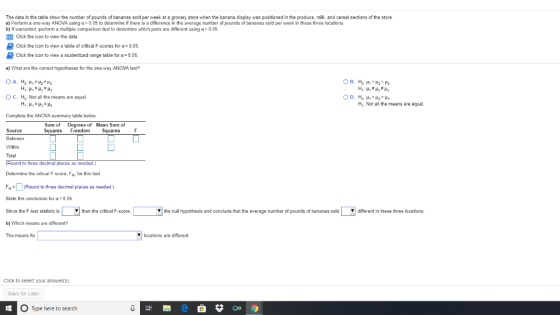
Number of Pounds of Bananas Sold Produce (1Milk Cereal 35 42 38 47 39 30 35 47 36 41 29 Print Done esis and conclude that the average number of pounds of bananas sold different in these three locations. The data in the table show the number of pounds of bananas sold per week at a grocery store when the banana display was positioned in the produce, milk, and cereal sections of the store a) Perform a one-way ANOVA using α= 0 05 to determine if there is a difference in the average number of pounds of bananas 9old per week in these three locations b) If warranted, perform a multiple comparison test to determine which pairs are different using a 0.05 Click the icon to view the data Click the icon to view a table of critical F-scores for α-o05 Click the icon to view a studentized range table for α: 0.05 a) What are the correct hypotheses for the one-way ANOVA test? C. Ho' Not all the means are equal H Not all the means are equal. Complate the ANOVA summary table below Sum of Degrees of Mean Sum of Squares Freedom Squares F Source Belween Within Total d to three decimal places as needed) Determine the critical F-score, Fa, for this test Round to three decimal places as needed) State the conclusion for α 0 05 Since the F-test statistic is b) Which means are different? The means for than the critical F-gcore ▼ the null hypothesis and conclude that the average number of pounds of bananas sold | ▼| different in these three locations. locations are different. click to select your answers) Save for Later O Type here to search

Answer 1

D)

P(1)	M(2)	C(3)		Anova: Single Factor
38	35	35
47	47	42		SUMMARY
39	36	44		Groups	Count	Sum	Average	Variance
30	41	29		P(1)	4	154	38.5	48.33333
	44			M(2)	5	203	40.6	26.3
				C(3)	4	150	37.5	47
				ANOVA
				Source of Variation	SS	df	MS	F	P-value	F crit
				Between Groups	22.8	2	11.4	0.291	0.753	4.103
				Within Groups	391.2	10	39.12
				Total	414	12

F = 4.103

less, Fail to reject, not

b) Mean are not significantly different\

So there is NO mean which is different

NOTE=please provide the option for exact wording