Question

Using Matlab.

The following calibration data are from a hot wire anemometer (HWA) velocity measurement system for air flow: Air Velocity, V (m/s) HWA Output Voltage (E) 0.0 1.100 1. 1.1 1.362 2. 1.431 1.5 3. 1.487 2.0 4. 1.535 2.5 5. 1.576 6 3.0 1.647 4.0 7. 1.706 8. 5.0 1.780 9. 6.5 1.841 10. 8.0 1.910 10 11. 1.983 12. 13 13. 16 2.072 14. 20 2.159 15. 25 2.257 16. 32 2.379 17. 40 2.500 1. Perform a polynomial curve fit to the data using Matlab's polyfit command to obtain best fit for air velocity V as a function of voltage E: V(E). Plot the data points along with your curve fit. Justify the polynomial order that you have chosen. 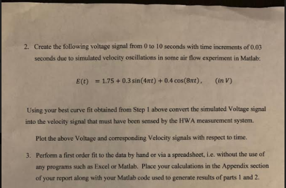curve 2. Create the following voltage signal from 0 to 10 seconds with time increments of 0.03 seconds due to simulated velocity oscillations in some air flow experiment in Matlab: 1.75+0.3 sin(47t) + 0.4 cos(8nt), (in V) E(t) Using your best curve fit obtained from Step 1 above convert the simulated Voltage signal into the velocity signal that must have been sensed by the HWA measurement system. Plot the above Voltage and corresponding Velocity signals with respect to time. 3. Perform a first order fit to the data by hand or via a spreadsheet, i.e. without the use of any programs such as Excel or Matlab. Place your calculations in the Appendix section of your report along with your Matlab code used to generate results of parts 1 and 2

Answer 1

V=[0 1.1 1.5 2.0 2.5 3.0 4.0 5.0 6.5 8.0 10 13 16 20 25 32 40]
E=[1.100 1.362 1.431 1.487 1.535 1.576 1.647 1.706 1.780 1.841 1.910 1.983 2.072 2.159 2.257 2.379 2.500]
P=polyfit(E,V,2);
fprintf('2nd degree Interpolated Equation is V=(%d)*E^2+(%d)*E+(%d)',P)
figure(1)
plot(E,V,'*')
xlabel('E')
ylabel('V')
hold on
Vnew=polyval(P,E);
plot(E,Vnew,'--r')
hold off
i=1;
for t=0:0.03:10
Et(i)=1.75+0.3*sin(4*pi*t)+0.4*cos(8*pi*t);
i=i+1;
end

Velocity_signal=(26.3635)*Et.^2+(-67.7798)*Et+(43.89);
figure(2)
plot(Et,Velocity_signal,'*')
xlabel('Voltage signal(Et)')
ylabel('Velocity_signal')

OUTPUT---------------------------------------------------------------------------------------------------

V =

 Columns 1 through 7:

    0.00000    1.10000    1.50000    2.00000    2.50000    3.00000    4.00000

 Columns 8 through 14:

    5.00000    6.50000    8.00000   10.00000   13.00000   16.00000   20.00000

 Columns 15 through 17:

   25.00000   32.00000   40.00000

E =

 Columns 1 through 8:

   1.1000   1.3620   1.4310   1.4870   1.5350   1.5760   1.6470   1.7060

 Columns 9 through 16:

   1.7800   1.8410   1.9100   1.9830   2.0720   2.1590   2.2570   2.3790

 Column 17:

   2.5000

2nd degree Interpolated Equation is V=(26.3635)*E^2+(-67.7798)*E+(43.89)
35 30 25 15 10 5 1.5 2 2,5 LLI LO 40 20 A

25 20 15 5 C 1 1.2 1.4 1.6 1.8 2 2.2 Voltage signal(Et) Velocitysignal 10