Question

Bivariate Fit of NONFOOD PURCHASES By AGE 90 80 70 60 50 40 30 20 20 30 40 50 60 AGE -Linear Fit Linear Fit NONFOOD_PURCHASES = 12.956633 0.8136836 AGE Summary of Fit RSquare RSquare Adj Root Mean Square Error Mean of Response Observations (or Sum Wgts) 0.33852 0.336478 11.54086 39.1842 326 Lack Of Fit Analysis of Variance Sum of Source DF Squares Mean Square F Ratio 22084.6 165.8106 133.2 Prob > F .00011 Model 1 22084.562 Error 324 43154.032 C. 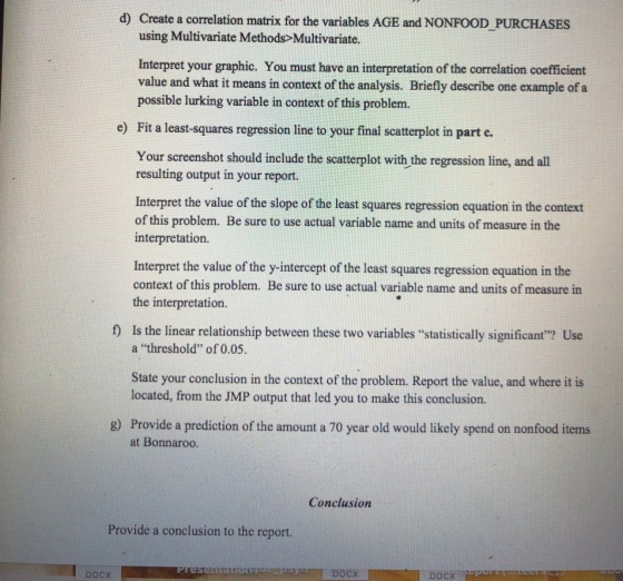Total 325 65238.594 Parameter Estimates Term Estimate Std Error t Ratio Prob>lt| 6.07 0001 12.88 0001 Intercept 12.956633 2.134756 AGE 0.8136836 0.06319 NONFOOD PURCHASES AN d) Create a correlation matrix for the variables AGE and NONFOOD PURCHASES using Multivariate Methods Multivariate. Interpret your graphic. You must have an interpretation of the correlation coefficient value and what it means in context of the analysis. Briefly describe one example of a possible lurking variable in context of this problem. e) Fit a least-squares regression line to your final scatterplot in part c. Your screenshot should include the scatterplot with the regression line, and all resulting output in your report. Interpret the value of the slope of the least squares regression equation in the context of this problem. Be sure to use actual variable name and units of measure in the interpretation. Interpret the value of the y-intercept of the least squares regression equation in the context of this problem. Be sure to use actual variable name and units of measure in the interpretation. f) Is the linear relationship between these two variables "statistically significant"? Use a threshold" of 0.05 State your conclusion in the context of the problem. Report the value, and where it is located, from the JMP output that led you to make this conclusion. g) Provide a prediction of the amount a 70 year old would likely spend on nonfood items at Bonnaroo. Conclusion Provide a conclusion to the report PresematcI rsy DOCX ce DOCX DOCX

Answer 1

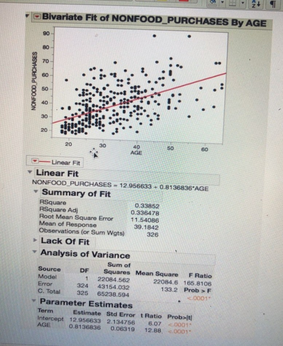
(d) scatter plot showed there is positive correlation(r) between the two variables as the points are concentrated on the line from quadrant III to quadrant I

correlation=r=sqrt(RSquare)=sqrt(0.33852)=0.5818

(e) here intercept=12.9566 which means if age is 0 then nonfood_purchase would be 12.9566 unit

and slope=0.8137 which means if age is increased to 1 unit then nonfood_purchase would increase 0.8137 unit and vice-versa

(f) yes, linear relationship between two variables is significant at alpha=5% as the p-value(<0.0001) of age is less than 0.05

(h)answer is 69.92

for age=70, the Nonfood_purchase=12.9566+0.8137*70=69.92 ( two decimal place approximation)