Consider the region of 1s resulting from the segmentation of the sparse regions in the ima...

Consider the region of 1s resulting from the segmentation of the sparse regions in the image of the Cygnus Loop in Example 10.24. Propose a technique for using this region as a mask to isolate the three main components of the image: (1) background, (2) dense inner region, and (3) sparse outer region.

EXAMPLE 10.24: Segmentation by region splitting and merging.

Figure 10.53(a) shows a 566 × 566 X-ray band image of the Cygnus Loop. The objective of this example is to segment out of the image the “ring” of less dense matter surrounding the dense center. The region of interest has some obvious characteristics that should help in its segmentation. First, we note that the data in this region has a random nature, indicating that its standard deviation should be greater than the standard deviation of the background (which is near 0) and of the large central region, which is fairly smooth. Similarly, the mean value (average intensity) of a region containing data from the outer ring should be greater than the mean of the darker background and less than the mean of the large, lighter central region. Thus, we should be able to segment the region of interest using the following predicate:

where m and σ are the mean and standard deviation of the pixels in a quadregion, and a and b are constants.

Analysis of several regions in the outer area of interest revealed that the mean intensity of pixels in those regions did not exceed 125 and the standard deviation was always greater than 10. Figures 10.53(b) through (d) show the results obtained using these values for a and b, and varying the minimum size allowed for the quadregions from 32 to 8. The pixels in a quadregion whose

FIGURE 10.53 (a) Image of the Cygnus Loop supernova, taken in the X-ray band by NASA’s Hubble Telescope. (b)-(d) Results of limiting the smallest allowed quadregion to sizes of 32 ×32, 16 ×16, and 8 × 8 pixels, respectively. (Original image courtesy of NASA.)

pixels satisfied the predicate were set to white; all others in that region were set to black. The best result in terms of capturing the shape of the outer region was obtained using quadregions of size 16 × 16. The black squares in Fig. 10.53(d) are quadregions of size 8 × 8 whose pixels did not satisfied the predicate. Using smaller quadregions would result in increasing numbers of such black regions. Using regions larger than the one illustrated here results in a more “blocklike” segmentation. Note that in all cases the segmented regions (white pixels) completely separate the inner, smoother region from the background. Thus, the segmentation effectively partitioned the image into three distinct areas that correspond to the three principal features in the image: background, dense, and sparse regions. Using any of the white regions in Fig. 10.53 as a mask would make it a relatively simple task to extract these regions from the original image (Problem 10.40). As in Example 10.23, these results could not have been obtained using edge- or threshold-based segmentation.

EXAMPLE 10.23: Segmentation by region growing.

Figure 10.51(a) shows an 8-bit X-ray image of a weld (the horizontal dark region) containing several cracks and porosities (the bright regions running horizontally through the center of the image). We illustrate the use of region growing by segmenting the defective weld regions. These regions could be used in applications such as weld inspection, for inclusion in a database of historical studies, or for controlling an automated welding system.

The first order of business is to determine the seed points. From the physics of the problem, we know that cracks and porosities will attenuate X-rays considerably less than solid welds, so we expect the regions containing these types of defects to be significantly brighter than other parts of the X-ray image. We can extract the seed points by thresholding the original image, using a threshold set at a high percentile. Figure 10.51(b) shows the histogram of the image and Fig. 10.51(c) shows the thresholded result obtained with a threshold equal to the 99.9 percentile of intensity values in the image, which in this case was 254 (see Section 10.3.5 regarding percentiles). Figure 10.51(d) shows the result of morphologically eroding each connected component in Fig. 10.51(c) to a single point.

FIGURE 10.51 (a) X-ray image of a defective weld. (b) Histogram. (c) Initial seed image. (d) Final seed image (the points were enlarged for clarity). (e) Absolute value of the difference between (a) and (c). (f) Histogram of (e). (g) Difference image thresholded using dual thresholds. (h) Difference image thresholded with the smallest of the dual thresholds. (i) Segmentation result obtained by region growing. (Original image courtesy of X-TEK Systems, Ltd.)

Next, we have to specify a predicate. In this example, we are interested in appending to each seed all the pixels that (a) are 8-connected to that seed and

(b) are “similar” to it. Using intensity differences as a measure of similarity, our predicate applied at each location (x, y)is

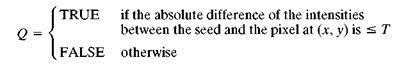
where T is a specified threshold. Although this predicate is based on intensity differences and uses a single threshold, we could specify more complex schemes in which a different threshold is applied to each pixel, and properties other than differences are used. In this case, the preceding predicate is sufficient to solve the problem, as the rest of this example shows.

From the previous paragraph, we know that the smallest seed value is 255 because the image was thresholded with a threshold of 254. Figure 10.51(e) shows the absolute value of the difference between the images in Figs. 10.51(a) and (c).The image in Fig. 10.51(e) contains all the differences needed to compute the predicate at each location (x, y). Figure 10.51(f) shows the corresponding histogram. We need a threshold to use in the predicate to establish similarity. The histogram has three principal modes, so we can start by applying to the difference image the dual thresholding technique discussed in Section 10.3.6. The resulting two thresholds in this case were T1 = 68 and T2 = 126, which we see correspond closely to the valleys of the histogram. (As a brief digression, we segmented the image using these two thresholds. The result in Fig. 10.51(g) shows that the problem of segmenting the defects cannot be solved using dual thresholds, even though the thresholds are in the main valleys.)

Figure 10.51(h) shows the result of thresholding the difference image with only T1. The black points are the pixels for which the predicate was TRUE; the others failed the predicate. The important result here is that the points in the good regions of the weld failed the predicate, so they will not be included in the final result. The points in the outer region will be considered by the region-growing algorithm as candidates. However, Step 3 will reject the outer points, because they are not 8-connected to the seeds. In fact, as Fig. 10.51(i) shows, this step resulted in the correct segmentation, indicating that the use of connectivity was a fundamental requirement in this case. Finally, note that in Step 4 we used the same value for all the regions found by the algorithm. In this case, it was visually preferable to do so.