Question

A state space linear system is shown below. Use Matlab to solve the following problems.

Requirement for project report: (1) Results; (2) Matlab code.

dx1/dt=-x1(t)+u(t)

dx2/dt=x1(t)-2x2(t)-x3(t)+3u(t)

dx3/dt=-3x3(t)

y(t)=-x1(t)+2x2(t)+x3(t)+u(t)

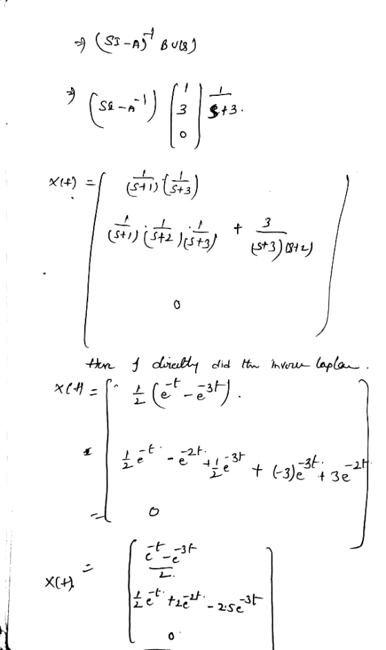
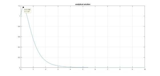
(1) Assume the system has input u(t)=e^-3t if t>t₀ and zero initial state x(0)=[0;0;0]. Using the transition matrix obtained, compute the system’s output (analytical solution), and plot the output as a function of time (t within 0 to 10).

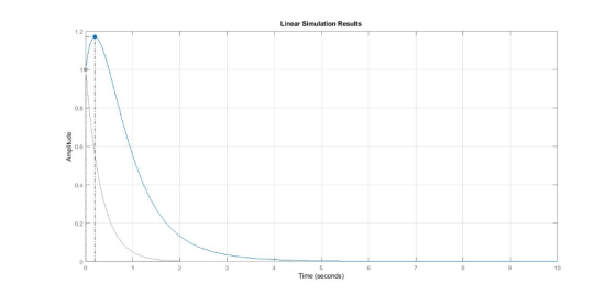
(2) Using the function lsim to simulate the system’s output (analytical solution), and plot the output as a function of time (t within 0 to 10). The system has input (u(t)=e^-3t if t>0) and zero initial state x(0)=[0;0;0] .

(3) Compare results for Question (1) and (2).

Answer 1

S(st3 ss-A) ISL-A 0

Ce XCH)

Ce XCH)

matlab code:

clc;clear all;close all;
t=0:0.001:10;
y=0.5*(exp(-t))+4*(exp(-2*t))-3.5*(exp(-3*t)); % analytical solution
figure
plot(t,y),grid; %plot of the analytical solution
title('analytical solution')
A=[-1 0 0;1 -2 -1;0 0 -3]
B=[1;3;0]
C=[-1 2 1]
D=[1]
sys=ss(A,B,C,D)
ip=exp(-3*t);
figure
lsim(sys,ip,t),grid

analytical solution 1.2 X:0.195 Y: 1.17 0.8 0.6 0.4 0.2 10

Linear Simulation Results 0.8 0.6 0.4 0.2 10 Time (seconds)