Question

A researcher is examining the effect of number of years in a particular job (tenure) on the hourly wage (USD) earned. She estimates two regression models using data on 124 young women surveyed in 1988. In the first regression, she regressed logged hourly wage on logged tenure in the current job (years in current job). In the second regression she regressed logged hourly wage on logged tenure in the current job, as well as age, total years of schooling completed, and total years of work experience (in any job).

reg ln_wage ln_tenure Source SS df MS 124 18.61 1 Model Residual 1 4.96082255 32.5291117 4.96082255 .266632063 Number of obs F(1, 122) Prob > F R-squared Adj R-squared Root MSE 122 0.0000 0.1323 0.1252 .51636 Total 37.4899342 123 .304796213 in_wage 1 Coef. Std. Err. t P>t] [95% Conf. Interval] 4.31 In_tenure | _cons . 163222 1.641472 .0378406 .0704397 0.000 0.000 0883128 1.50203 .2381313 1.780915 23.30 · reg ln_wage ln_tenure age yrs_school experience Source SS df MS = 124 10.45 4 Modell Residual 9.7457874 27.7441468 2.43644685 .233144091 Number of obs F(4, 119) Prob > F R-squared Adj R-squared Root MSE 119 = 0.0000 0.2600 0.2351 .48285 Total 1 37.4899342 123 .304796213 In_wage 1 Coef. Std. Err. t P>t [95% Conf. Interval] ln_tenure age yrs_school experience _cons .0959318 .0081925 .0542063 .0291484 .3300737 .0418616 .0147956 .0154112 .0121425 .6275823 2.29 0.55 3.52 2.40 0.53 0.024 0.581 0.001 0.018 0.600 .0130417 -.0211043 .0236905 .0051049 -.912602 . 1788219 .0374894 .0847221 .0531918 1.572749

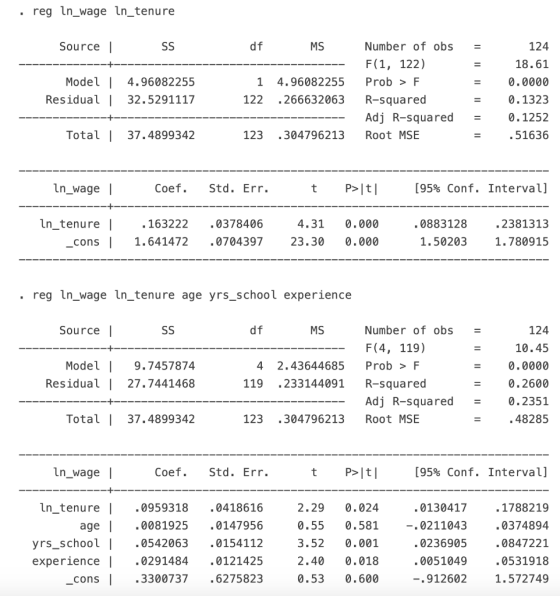
a)What is the interpretation of the coefficient estimate of 0.0959318 in the second regression?

b)The coefficient on logged job tenure is much lower in the second regression compared to the first one. Why? Answer with 2-3 sentences.

c)Find the t-statistic of 0.55 and the associated p-value of 0.581 reported in the output for the second regression. What formula was used to calculate this test statistic? Also, identify the values that were used for the components of this formula. Lastly, what are the set of hypotheses that go with the p-value?

Answer 1

DATE Here on we have in response and we have un for predicter so approximation method which says If en (y) = pot fun (8,2) when x increase by yl by 14. Then y increase by litool) p2 times increase by Il Now Here tenure wage increase by (1 torol Co.o955) = 0.096 regression considered slope is مبل هابيا In 1st have Only I vorable so hare highey but construct and regression we have considered more Vanable, to variation is distributed in and among regassion regressors Estat = coefficient SE Estat = 0.00819 0.55 000147 and hypotheis is Ho? B3=0, H, 133 33 ? slope of age