Question

Assignment 1: PID tuning 1. Use the Ziegler-Nichols method to get an initial tuning of a PID controller that improves the response of a svstem represented by the following openloop dynamics 0.75 s G(s) (s + 10)(s +1)s2 2. What is the cross over frequency, gain margin, and phase mar- gin of the uncompensated system? 3. Compare the cross over frequency, gain margin, and phase 4. Compare the step responses of both. Indicate how you gener- 5. How would you tune the PID gains further? Explain your margin with the PID compensated system. ated these responses. approach with Bode plots and step response

Answer 1

Answer:-

(1)

PID controller design:

increase the gain for the step response of the system such that the system oscillates . that gain is Km and the frequency of oscillations is Wm.

s=tf('s');
g=0.75*s/(s^2*(s+1)*(s+10));
sisotool(g)

The PID controller is

Kp= 0.6* 60 = 36

Kd= 86.25

Ki=3.75

the controller is Gc = Kp + Ki / s + Kd s

(2)

margins and cross over frequencies of uncompensated system

s=tf('s');
g=0.75*s/(s^2*(s+1)*(s+10));
margin(g)

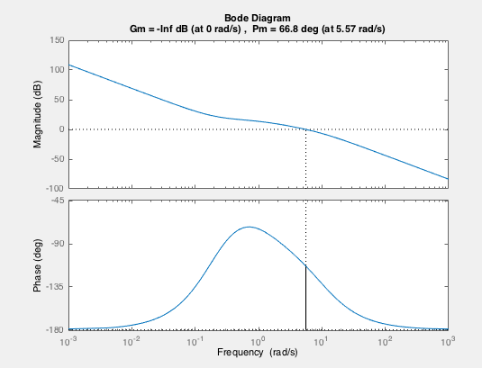
(3)

margins and cross over frequencies of compensated system

s=tf('s');
g=0.75*s/(s^2*(s+1)*(s+10));
gc=36+86.25*s+(3.75/s);

margin(g)

figure
margin(g*gc)

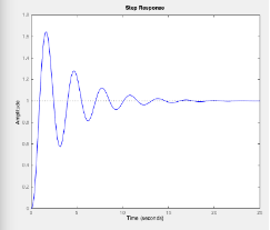
(4)

step response of the sysetms:

s=tf('s');
g=0.75*s/(s^2*(s+1)*(s+10));
gc=36+86.25*s+(3.75/s);
step(feedback(g,1),feedback(g*gc,1))
legend('uncompensated system ' , 'compensated system')

(5)

the PID gains can be tuned further based on the requirements like settling time ,proper damping ,overshoot