
Homework Answers
Add Answer to:
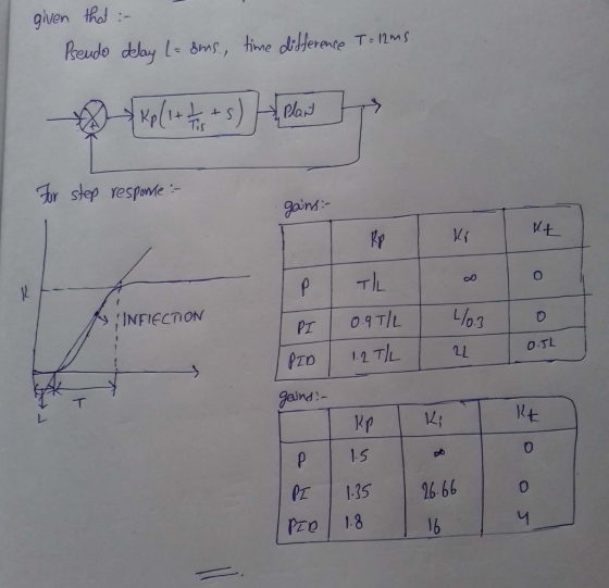
Problem #3: For an open-loop step response that yields the following data: Pseudo delays 8 ms and time difference T·12 ms. a) Find the PID Control gains using Zeigler-Nichols tuning method....
Problem #2: For experimental test data, you have a system with the following unit step responses. 1.0 0.8 0.6 0.4 0.2 0123456789 10 Time (sec) a) b) Determine the response's time delay and t...
 Problem #2: For experimental test data, you have a system with the following unit step responses. 1.0 0.8 0.6 0.4 0.2 0123456789 10 Time (sec) a) b) Determine the response's time delay and tangential slope along the transient response. Find the PID Control gains using Zeigler-Nichols tuning method.
Problem #2: For experimental test data, you have a system with the following unit step responses. 1.0 0.8 0.6 0.4 0.2 0123456789 10 Time (sec)
a) b) Determine the response's time delay...
Problem #2: For experimental test data, you have a system with the following unit step responses. 1.0 0.8 0.6 0.4 0.2 0123456789 10 Time (sec) a) b) Determine the response's time delay and tangential slope along the transient response. Find the PID Control gains using Zeigler-Nichols tuning method.
Problem #2: For experimental test data, you have a system with the following unit step responses. 1.0 0.8 0.6 0.4 0.2 0123456789 10 Time (sec)
a) b) Determine the response's time delay...
For the open loop response shown, find the ZN tuning parameters assuming that the step response...
 For the open loop response shown, find the ZN tuning parameters assuming that the step response change is 10. pR 1.8 1.6 1.4 Assume step response amplitude change 10 A step response 10 1.2 0.8 0.6 APV 0.4 0.2 -0.2 0 1 23 4 5 7 Te d 11 13 15 17 19 From the process reaction curve determine the dead time, td, the time constant or time for the response to change, Tm, the ultimate value that the response...
Response with lines drawn is shown as the second graph, both graphs are the exact same. ANSWER PART (a) open-loop tr...
 Response with lines drawn is shown as the second graph, both
graphs are the exact same.
ANSWER PART (a)
open-loop transient response A PID controller for a process is to be tuned by carrying out an test. The system control temperature varies from 25 °C to 300 °C with a 200 °C setpoint. The output of the PID controller is a heater control voltage ranging from 0 VAC to 240 VAC. The test is started by having a 150 VAC...
Response with lines drawn is shown as the second graph, both
graphs are the exact same.
ANSWER PART (a)
open-loop transient response A PID controller for a process is to be tuned by carrying out an test. The system control temperature varies from 25 °C to 300 °C with a 200 °C setpoint. The output of the PID controller is a heater control voltage ranging from 0 VAC to 240 VAC. The test is started by having a 150 VAC...
uestion 14 The reaction curve for a heating process is shown below. Using the graph shown and the open loop Ziegler Find Kd for the PID controller Nichlos method 40 Input Step change 20 10 0 10 2...
 uestion 14 The reaction curve for a heating process is shown below. Using the graph shown and the open loop Ziegler Find Kd for the PID controller Nichlos method 40 Input Step change 20 10 0 10 20 30 40 S0 0 Time (sec)
uestion 14 The reaction curve for a heating process is shown below. Using the graph shown and the open loop Ziegler Find Kd for the PID controller Nichlos method 40 Input Step change 20 10 0...
uestion 14 The reaction curve for a heating process is shown below. Using the graph shown and the open loop Ziegler Find Kd for the PID controller Nichlos method 40 Input Step change 20 10 0 10 20 30 40 S0 0 Time (sec)
uestion 14 The reaction curve for a heating process is shown below. Using the graph shown and the open loop Ziegler Find Kd for the PID controller Nichlos method 40 Input Step change 20 10 0...
PLEASE DO IN MATLAB Problem 8 (PID feedback control). This problem is about Proportional-Integral-Derivative feedback control...
 PLEASE DO IN MATLAB
Problem 8 (PID feedback control). This problem is about Proportional-Integral-Derivative feedback control systems. The general setup of the system we are going to look at is given below: e(t) u(t) |C(s) y(t) P(s) r(t) Here the various signals are: signal/system r(t) y(t) e(t) P(s) C(s) и(t) meaning desired output signal actual output signal error signal r(t) y(t) Laplace transform of the (unstable) plant controller to be designed control signal Our goal is to design a controller...
PLEASE DO IN MATLAB
Problem 8 (PID feedback control). This problem is about Proportional-Integral-Derivative feedback control systems. The general setup of the system we are going to look at is given below: e(t) u(t) |C(s) y(t) P(s) r(t) Here the various signals are: signal/system r(t) y(t) e(t) P(s) C(s) и(t) meaning desired output signal actual output signal error signal r(t) y(t) Laplace transform of the (unstable) plant controller to be designed control signal Our goal is to design a controller...
For the closed-loop system shown, and given: C(s) 8.41 s+8.10 G(8 2 0.02 3.00 2out G(s) C(s) control plant Part A-Plant 1% settling time Find the 1% settling time of the plant G(s) to a unit step inp...
 For the closed-loop system shown, and given: C(s) 8.41 s+8.10 G(8 2 0.02 3.00 2out G(s) C(s) control plant Part A-Plant 1% settling time Find the 1% settling time of the plant G(s) to a unit step input. 15.38 t,3% - Submit X ncorrect; Try Again - Part B Plant: Overshoot Find the overshoot of the plant G(s)to a unit step input. Give your answer as a percentage Mp: | Value Units Submit Request Answer Part C - Closed-loop system:...
Problem 8-1 Consider the following time series data. Week Value 1 18 2 12 3 16...
 Problem 8-1 Consider the following time series data. Week Value 1 18 2 12 3 16 4 5 6 11 1914 Using the naïve method (most recent value) as the forecast for the next week, compute the following measures of forecast accuracy. (a) Mean absolute error If required, round your answer to one decimal place. (b) Mean squared error If required, round your answer to one decimal place. (c) Mean absolute percentage error If required, round your intermediate calculations and...
2. Create a main program that calls the subroutine created on problem 1 and compare results using the following data sets: b. 1 5), (0, 8), (3,-10) С. (-10,-2), (45), (73), (12, 20) t: (c...
 2. Create a main program that calls the subroutine created on problem 1 and compare results using the following data sets: b. 1 5), (0, 8), (3,-10) С. (-10,-2), (45), (73), (12, 20) t: (copy and paste the output in the following box) Use MATLAB or Scilab to solve the following problems 1. Create a MATLAB subroutine called Lagrange.m that receives two set data points, x and y and plots the curve by interpolating the missing points (hEX-Xi-1) using Lagrange...
 Problem #2: For experimental test data, you have a system with the following unit step responses. 1.0 0.8 0.6 0.4 0.2 0123456789 10 Time (sec) a) b) Determine the response's time delay and tangential slope along the transient response. Find the PID Control gains using Zeigler-Nichols tuning method.
Problem #2: For experimental test data, you have a system with the following unit step responses. 1.0 0.8 0.6 0.4 0.2 0123456789 10 Time (sec)
a) b) Determine the response's time delay...
Problem #2: For experimental test data, you have a system with the following unit step responses. 1.0 0.8 0.6 0.4 0.2 0123456789 10 Time (sec) a) b) Determine the response's time delay and tangential slope along the transient response. Find the PID Control gains using Zeigler-Nichols tuning method.
Problem #2: For experimental test data, you have a system with the following unit step responses. 1.0 0.8 0.6 0.4 0.2 0123456789 10 Time (sec)
a) b) Determine the response's time delay...
 For the open loop response shown, find the ZN tuning parameters assuming that the step response change is 10. pR 1.8 1.6 1.4 Assume step response amplitude change 10 A step response 10 1.2 0.8 0.6 APV 0.4 0.2 -0.2 0 1 23 4 5 7 Te d 11 13 15 17 19 From the process reaction curve determine the dead time, td, the time constant or time for the response to change, Tm, the ultimate value that the response...
 Response with lines drawn is shown as the second graph, both
graphs are the exact same.
ANSWER PART (a)
open-loop transient response A PID controller for a process is to be tuned by carrying out an test. The system control temperature varies from 25 °C to 300 °C with a 200 °C setpoint. The output of the PID controller is a heater control voltage ranging from 0 VAC to 240 VAC. The test is started by having a 150 VAC...
Response with lines drawn is shown as the second graph, both
graphs are the exact same.
ANSWER PART (a)
open-loop transient response A PID controller for a process is to be tuned by carrying out an test. The system control temperature varies from 25 °C to 300 °C with a 200 °C setpoint. The output of the PID controller is a heater control voltage ranging from 0 VAC to 240 VAC. The test is started by having a 150 VAC...
 uestion 14 The reaction curve for a heating process is shown below. Using the graph shown and the open loop Ziegler Find Kd for the PID controller Nichlos method 40 Input Step change 20 10 0 10 20 30 40 S0 0 Time (sec)
uestion 14 The reaction curve for a heating process is shown below. Using the graph shown and the open loop Ziegler Find Kd for the PID controller Nichlos method 40 Input Step change 20 10 0...
uestion 14 The reaction curve for a heating process is shown below. Using the graph shown and the open loop Ziegler Find Kd for the PID controller Nichlos method 40 Input Step change 20 10 0 10 20 30 40 S0 0 Time (sec)
uestion 14 The reaction curve for a heating process is shown below. Using the graph shown and the open loop Ziegler Find Kd for the PID controller Nichlos method 40 Input Step change 20 10 0...
 PLEASE DO IN MATLAB
Problem 8 (PID feedback control). This problem is about Proportional-Integral-Derivative feedback control systems. The general setup of the system we are going to look at is given below: e(t) u(t) |C(s) y(t) P(s) r(t) Here the various signals are: signal/system r(t) y(t) e(t) P(s) C(s) и(t) meaning desired output signal actual output signal error signal r(t) y(t) Laplace transform of the (unstable) plant controller to be designed control signal Our goal is to design a controller...
PLEASE DO IN MATLAB
Problem 8 (PID feedback control). This problem is about Proportional-Integral-Derivative feedback control systems. The general setup of the system we are going to look at is given below: e(t) u(t) |C(s) y(t) P(s) r(t) Here the various signals are: signal/system r(t) y(t) e(t) P(s) C(s) и(t) meaning desired output signal actual output signal error signal r(t) y(t) Laplace transform of the (unstable) plant controller to be designed control signal Our goal is to design a controller...
 For the closed-loop system shown, and given: C(s) 8.41 s+8.10 G(8 2 0.02 3.00 2out G(s) C(s) control plant Part A-Plant 1% settling time Find the 1% settling time of the plant G(s) to a unit step input. 15.38 t,3% - Submit X ncorrect; Try Again - Part B Plant: Overshoot Find the overshoot of the plant G(s)to a unit step input. Give your answer as a percentage Mp: | Value Units Submit Request Answer Part C - Closed-loop system:...
 Problem 8-1 Consider the following time series data. Week Value 1 18 2 12 3 16 4 5 6 11 1914 Using the naïve method (most recent value) as the forecast for the next week, compute the following measures of forecast accuracy. (a) Mean absolute error If required, round your answer to one decimal place. (b) Mean squared error If required, round your answer to one decimal place. (c) Mean absolute percentage error If required, round your intermediate calculations and...
 2. Create a main program that calls the subroutine created on problem 1 and compare results using the following data sets: b. 1 5), (0, 8), (3,-10) С. (-10,-2), (45), (73), (12, 20) t: (copy and paste the output in the following box) Use MATLAB or Scilab to solve the following problems 1. Create a MATLAB subroutine called Lagrange.m that receives two set data points, x and y and plots the curve by interpolating the missing points (hEX-Xi-1) using Lagrange...
Most questions answered within 3 hours.
-
The average length of time between arrivals at a turnpike
toll-booth is 26 seconds. What is...
asked 1 hour ago -
(a) A piston at 6.1 atm contains a gas that occupies a volume of
3.5 L....
asked 2 hours ago -
Please answer true or false. Words
cannot be changed or added in to make it true...
asked 2 hours ago -
An empty test tube weighs 15.923 grams. Then,
MgCl2•6H2O is added into the test tube. After...
asked 2 hours ago -
Assume memory access is 10 units of time and disk access is
10000 units of time....
asked 2 hours ago -
1. Are all good samples random?
2. Magazines often report surveys giving statistics such as “63%...
asked 3 hours ago -
Under all the various types of market structures, firms
must eventually earn some economic profits for...
asked 3 hours ago -
Consider the following fitness regime for a single locus trait
with two co-dominant alleles: w11 =...
asked 3 hours ago -
A large cable company reports the following.
80% of its customers subscribe to its cable TV...
asked 3 hours ago -
Please answer the question in brief.
Discuss the role of ERP in organizations. Are ERP tools...
asked 3 hours ago -
Discuss the pros and cons of collaborative software such
as SameTime. Does it increase productivity? What...
asked 3 hours ago -
Buying your in-laws a gift because it’s expected is
due to the ____________ motive of gift-giving....
asked 3 hours ago