Question

Can you solve the question CE 4-3. do not need to do #g & h.

CE4-2. Create a new workbook and take the following actions: a. Name and save your workbook using your own choosing b. Enter the value This is the content of cell C7 into cell C7. a name of c. Use F2 to change the value in cell C7 to This is part of the content of cell C7 d. Add the value January to cells B2 through B14. Key the data just E Add the alue lanvaryto cell C2. and the value February oell c NgImt botk. C3 and dras Explain what happens. once. cens C2 and dw to cell c14. f. Create a list of odd numbers from 1 to 11 in cells C3 through C8. Key only the values l and 3. Enter the value MIS 1 in cell D3 and the value drag the small black hoy down to cell D14. Pplain wtat happes. CE4-3. Click the tab named Sheet2 in the workbook you used for question 2. a. Place the labels Part Description, Quantity Cost, and Total Value in cells B2, C2, D2, and E2, re- on Hand spectively. Center each label in its cell and make the labels bold. (Do this by highlighting the labels and clicking the bold B in the Font section of the Home tab.) Make each column large enough to show the entire label after formatting. 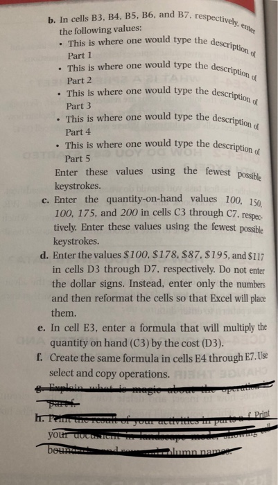b. In cells B3, B4, B5, B6, and B7. respectively. enter the following values: This is where one would type the description of Part 1 This is where one would type the description of Part 2 one would type the description of This is where Part 3 This is where one would type the description of Part 4 This is where one would type the description of e Part 5 Enter these values using the fewest p0ssil UOY O W keystrokes. c. Enter the quantity-on-hand values 100. 150 100, 175, and 200 in cells C3 through C7, respec tively. Enter these values using the fewest possible keystrokes. d. Enter the values $100, $178, $87, $195, and $117 in cells D3 through D7, respectively. Do not enter the dollar signs. Instead, enter only the numbers and then reformat the cells so that Excel will place them. e. In cell E3, enter a formula that will multiply the MAquantity on hand (C3) by the cost (D3). f. Create the same formula in cells E4 through E7. Use select and copy operations. T Lplain magic abou swbet- h. e in Print your boun COCt.ICn d ra alumn name

Answer 1

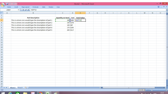
The followings are the screenshots of the work -

Formulas Review View Data Page Layout Insert Home D12 B A 1 Quantity on Hand Cost Total Value Part Description 2. This is where one would type the description of part 1 3 This is where one would type the description of part 2 This is where one would type the description of part 3 This is where one would type the description of part 4 4 5 6 This is where one would type the description of part 5 7 8 9 10 11 12 13 14 15 17 18 19 20 21 22 23 24 25 26 27 28 29 sheet2 Sheet3 100 % ( ) 4 23:10 Ready ENG 15/06/2019

For Creating bold and centered aligned headings, first write the content into cells from B2 to E2. Then select these cells, go to home, select bold (or press clt+B) and select center text alignment.

Now, for using least keystrok for filling values from B3 to B7, first write in B3 cell, then write "thi" in B4, it will automatically make the whole senyence of B3 appear in B4, then press enter. Afterwards double click in cell B4 and write 2 deleting 1. Then select B3 and B4 and drag the + sign on bottom right corner to cell B7.

c) Now enter the values -

After writing the values in Cost, without dollar sign, select the values from cells D3 to D7, then go to home, select currency and it will change to dollar.

Microsoft Excel Book2 Page Layout Home Insert Formulas Data Review View E AutoSum Cut Calibri Wrap Text A A 11 Fill Ea Copy General Paste BI U Format Cell Styles Merge & Center ABC 123 Insert Delete Forma Sort & Find & Format Painter Clear format Select Shyle Clipboard Font Alignment Cells Editing Number 100 $100 150 $178 100 $87 175 $195 200 $117 This is where one would type the description of part 1 3 12 S1 This is where one would type the description of part 2 4 Currency 5 This is where one would type the description of part 3 This is where one would type the description of part 4 $100 6 7 This is where one would type the description of part 5 Accounting $100 8 9 Short Date 10 $100 11 Long Date 12 $100 13 Time $100 Percentage 16 $100 17 18 Fraction $100 19 20 Scientifie 10 21 $100 22 More Number Formats.. 23 24 25 26 27 28 29 i4 Sheet3 a Sheet2 10096 Count: 5 Ready 23:19

d) In cell E3 write"=C3*D3" and press enter. Then drag the cell E3 till E7 to get values as follows -

Microsoft Excel Book2 Home Insert Page Layout Formulas Data Review View f D3°C3 LINEST B A C D M N C 1 Total Value Part Description Quantity on Hand Cost 100 $100D3*c3 This is where one would type the description of part 1 3 150 $178 This is where one would type the description of part 2 This is where one would type the description of part 3. 4 100 $87 5 175 $195 This is where one would type the description of part 4 6 200 $117 7 This is where one would type the description of part 5 9 10 11 12 13 16 17 18 19 20 21 22 23 24 25 26 27 28 29 i4 Sheet3 sheet2 100%(- Edit 23:23

n Microsoft Excel Book2 Home Insert Page Layout Formulas Data Review View ( X v F19 D A C G M N C 1 Part Description Quantity on Hand Cost Total Value 2 This is where one would type the description of part 1 100 $100 $10,000 3 150 $178 $26,700 This is where one would type the description of part 2 This is where one would type the description of part 3 4 100 $87 $8.700 5 175 $195 $34,125 This is where one would type the description of part 4 6 200 $117 $23.400 7 This is where one would type the description of part 5 9 10 11 12 13 16 17 18. 19 20 21 22 23 24 25 26 27 28 29 i4 Sheet3 a sheet2 Enter 23:25