Question

in MATLAB

Curve fitting

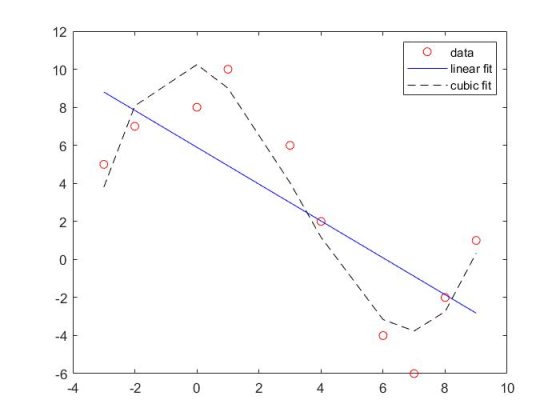
Given the following data, find the best linear functional relationship and cubic functional relationship using “polyfit,” “polyval,” and “plot” built-in functions. Plot all three fits that you got from Matlab. A rough plot by hand is allowable. You do not need to provide any codes.

     x = [-3, -2, 0, 1, 3, 4, 6, 7, 8, 9];

     y = [5, 7, 8, 10, 6, 2, -4, -6, -2, 1];

Answer 1

Code:

clc
clear

x = [-3, -2, 0, 1, 3, 4, 6, 7, 8, 9];
y = [5, 7, 8, 10, 6, 2, -4, -6, -2, 1];

pl = polyfit(x, y, 1);
yl = polyval(pl,x);

pc = polyfit(x, y, 3);
yc = polyval(pc,x);

plot(x, y, 'ro');
hold on
plot(x, yl, 'b-');
plot(x, yc, 'k--')
legend('data', 'linear fit', 'cubic fit')

Output:

o data linear fit ---.cubic fit -2 0 2 4 6 8 10