
MATLAB Code. Try not to use SYMS package as it does not load on Octave.
Homework Answers
I'm providing the screenshots of the work please do follow them and please do upvote thank you.
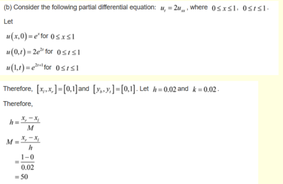
![(«,,x,]= [0,1] and [yo,y;] = [0,1]. Let h=0.02 and k = 0.02. Therefore, h=*, -X M M=*, -X, h 1-0 0.02 = 50 Similarly, k =); N](http://img.homeworklib.com/questions/ce3bfd20-0029-11eb-af00-355dccf2fffa.png?x-oss-process=image/resize,w_560)

Add Answer to:
MATLAB Code. Try not to use SYMS package as it does not load on
Octave.
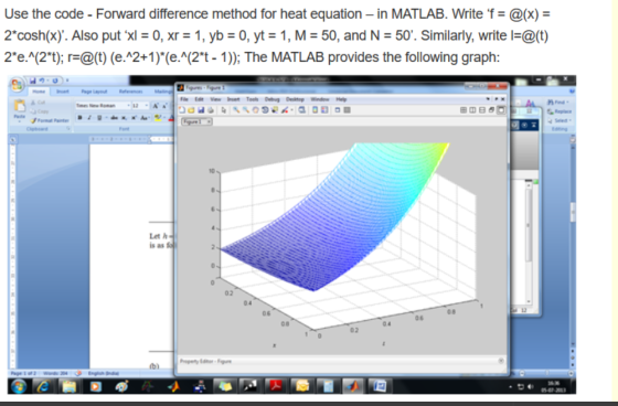
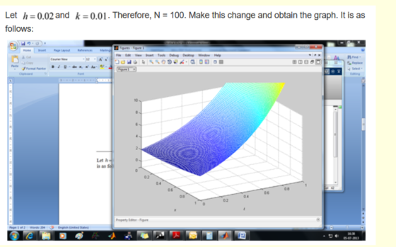
Use...
Please do not use SYMS package. It does not work on Octave for me. Matlab code...
 Please do not use SYMS package. It does not work on Octave for
me.
Matlab code needed for: 1. Apply the Explicit Trapezoid Method on a grid of step size h = 0.1 in [0, 1] to the initial value problems in Exercise 1. Print a table of the t values, approximations, and global truncation error at each step. IVP (Exercise 1): (a) y'=1 (b) y' = 12y (c) y' = 2(t+1)y (d) y = 564, (e) y'=1/y² (1) y'=1/y2...
Please do not use SYMS package. It does not work on Octave for
me.
Matlab code needed for: 1. Apply the Explicit Trapezoid Method on a grid of step size h = 0.1 in [0, 1] to the initial value problems in Exercise 1. Print a table of the t values, approximations, and global truncation error at each step. IVP (Exercise 1): (a) y'=1 (b) y' = 12y (c) y' = 2(t+1)y (d) y = 564, (e) y'=1/y² (1) y'=1/y2...
Please use MATLAB, screenshot code and results An automotive power train control system is described by...
 Please use MATLAB, screenshot code and results
An automotive power train control system is described by the following matrix equations 1-12 -10 -57 [1] x= 1 0 0 +0 u To 100 y(t) = [ 35 – 5]x where u = -KX+r, and r is a unit step input. Use MATLAB/SIMULINK to plot different responses of the system output Y for the following feedback control gain matrix K: Casel: K = [1 44 67] Case2: K = [10 44 67]...
Please use MATLAB, screenshot code and results
An automotive power train control system is described by the following matrix equations 1-12 -10 -57 [1] x= 1 0 0 +0 u To 100 y(t) = [ 35 – 5]x where u = -KX+r, and r is a unit step input. Use MATLAB/SIMULINK to plot different responses of the system output Y for the following feedback control gain matrix K: Casel: K = [1 44 67] Case2: K = [10 44 67]...
please use octave calculator or matlab to answer (a)(ii)and(iii) 2. (a) Use Octave as a Calculator1 to answer this question. Suppose that A and B are two 8 × 9 matrices. The (i, j)-entry of the matri...
 please use octave calculator or matlab to answer
(a)(ii)and(iii)
2. (a) Use Octave as a Calculator1 to answer this question. Suppose that A and B are two 8 × 9 matrices. The (i, j)-entry of the matrix B is given by i *j -1. The (i, j)-entry of the matrix A equals 0 if i + j is divisible by 5 and equals the (i, j)-entry of the matrix B otherwise. i. What are the rank and nullity of matrices...
please use octave calculator or matlab to answer
(a)(ii)and(iii)
2. (a) Use Octave as a Calculator1 to answer this question. Suppose that A and B are two 8 × 9 matrices. The (i, j)-entry of the matrix B is given by i *j -1. The (i, j)-entry of the matrix A equals 0 if i + j is divisible by 5 and equals the (i, j)-entry of the matrix B otherwise. i. What are the rank and nullity of matrices...
SOLVE USING MATLAB ONLY AND SHOW FULL CODE. PLEASE TO SHOW TEXT BOOK SOLUTION. SOLVE PART D ONLY
 SOLVE USING MATLAB ONLY AND SHOW FULL CODE. PLEASE TO SHOW
TEXT BOOK SOLUTION. SOLVE PART D ONLY
Apply Euler's Method with step sizes h # 0.1 and h 0.01 to the initial value problems in Exercise 1. Plot the approximate solutions and the correct solution on [O, 1], and find the global truncation error at t-1. Is the reduction in error for h -0.01 consistent with the order of Euler's Method? REFERENCE: Apply the Euler's Method with step size...
SOLVE USING MATLAB ONLY AND SHOW FULL CODE. PLEASE TO SHOW
TEXT BOOK SOLUTION. SOLVE PART D ONLY
Apply Euler's Method with step sizes h # 0.1 and h 0.01 to the initial value problems in Exercise 1. Plot the approximate solutions and the correct solution on [O, 1], and find the global truncation error at t-1. Is the reduction in error for h -0.01 consistent with the order of Euler's Method? REFERENCE: Apply the Euler's Method with step size...
Matlab & Differential Equations Help Needed I need help with this Matlab project for differential equations. I've got 0 experience with Matlab other than a much easier project I did in another...
 Matlab & Differential Equations Help Needed
I need help with this Matlab project for differential equations.
I've got 0 experience with Matlab other than a much easier project
I did in another class a few semesters ago. All we've been given is
this piece of paper and some sample code. I don't even know how to
begin to approach this. I don't know how to use Matlab at all and I
barely can do this material.
Here's the handout:
Here's...
Matlab & Differential Equations Help Needed
I need help with this Matlab project for differential equations.
I've got 0 experience with Matlab other than a much easier project
I did in another class a few semesters ago. All we've been given is
this piece of paper and some sample code. I don't even know how to
begin to approach this. I don't know how to use Matlab at all and I
barely can do this material.
Here's the handout:
Here's...
Solve using Matlab Use the forward Euler method, Vi+,-Vi+(4+1-tinti ,Vi) for i= 0,1,2, , taking yo y(to) to be the initial condition, to approximate the solution at t-2 of the IVP y'=y-t2 + 1, 0-...
 Solve using Matlab
Use the forward Euler method, Vi+,-Vi+(4+1-tinti ,Vi) for i= 0,1,2, , taking yo y(to) to be the initial condition, to approximate the solution at t-2 of the IVP y'=y-t2 + 1, 0-t-2, y(0) = 0.5. Use N = 2k, k = 1, 2, , 20 equispaced time steps (so to = 0 and tN-1 = 2). Make a convergence plot, computing the error by comparing with the exact solution, y: t1)2 -exp(t)/2, and plotting the error as...
Solve using Matlab
Use the forward Euler method, Vi+,-Vi+(4+1-tinti ,Vi) for i= 0,1,2, , taking yo y(to) to be the initial condition, to approximate the solution at t-2 of the IVP y'=y-t2 + 1, 0-t-2, y(0) = 0.5. Use N = 2k, k = 1, 2, , 20 equispaced time steps (so to = 0 and tN-1 = 2). Make a convergence plot, computing the error by comparing with the exact solution, y: t1)2 -exp(t)/2, and plotting the error as...
the code in the photo for this I.V.P dy/dx= x+y. y(0)=1 i need the two in the photo thank you New folder Bookmark...
 the code in the photo for this I.V.P
dy/dx= x+y. y(0)=1
i need the two in the photo
thank you
New folder Bookmarks G Google dy/dx x+y, y(0)=1 2 h Exact Solution 1.8 Approximate Solution Mesh Points 1.6 -Direction Fied 1.4 1.2 1 0.8 04 0.2 0.3 0.1 0 X CAUsersleskandara\Desktop\New folder emo.m EDITOR PUBLISH VEW Run Section FILE NAVIGATE EDIT Breakpoints Run Run and FL Advance Run and Advance Time BREAKPOINTS RUN 1 - clear all 2 clc 3-...
the code in the photo for this I.V.P
dy/dx= x+y. y(0)=1
i need the two in the photo
thank you
New folder Bookmarks G Google dy/dx x+y, y(0)=1 2 h Exact Solution 1.8 Approximate Solution Mesh Points 1.6 -Direction Fied 1.4 1.2 1 0.8 04 0.2 0.3 0.1 0 X CAUsersleskandara\Desktop\New folder emo.m EDITOR PUBLISH VEW Run Section FILE NAVIGATE EDIT Breakpoints Run Run and FL Advance Run and Advance Time BREAKPOINTS RUN 1 - clear all 2 clc 3-...
6. Consider the Cauchy problem for the advection equation, u +cu0, where c>0 a) Expand u(z,t + k) in a Taylor series up to O(k3) terms. Then use the advection equation to obtain c2k2 uzz(x, t)...
 6. Consider the Cauchy problem for the advection equation, u +cu0, where c>0 a) Expand u(z,t + k) in a Taylor series up to O(k3) terms. Then use the advection equation to obtain c2k2 uzz(x, t) + O(k"). u(z, t + k) u(x, t) _ cku(x, t) +- b) Replace u and ur by centered difference approximations to obtain the explicit scheme This is the Lax-Wendroff method. It is von Neumann stable for 0 < 8 < 1 and it...
MATLAB help please!!!!! 1. Use the forward Euler method Vi+,-Vi + (ti+1-tinti , yi) for i=0.1, 2, , taking yo-y(to) to be the initial condition, to approximate the solution at 2 of the IVP y'=y-t...
 MATLAB help please!!!!!
1. Use the forward Euler method Vi+,-Vi + (ti+1-tinti , yi) for i=0.1, 2, , taking yo-y(to) to be the initial condition, to approximate the solution at 2 of the IVP y'=y-t2 + 1, 0 2, y(0) = 0.5. t Use N 2k, k2,...,20 equispaced timesteps so to 0 and t-1 2) Make a convergence plot computing the error by comparing with the exact solution, y: t (t+1)2 exp(t)/2, and plotting the error as a function of...
MATLAB help please!!!!!
1. Use the forward Euler method Vi+,-Vi + (ti+1-tinti , yi) for i=0.1, 2, , taking yo-y(to) to be the initial condition, to approximate the solution at 2 of the IVP y'=y-t2 + 1, 0 2, y(0) = 0.5. t Use N 2k, k2,...,20 equispaced timesteps so to 0 and t-1 2) Make a convergence plot computing the error by comparing with the exact solution, y: t (t+1)2 exp(t)/2, and plotting the error as a function of...
Problem 2 Wis) R(s) U(s) Gol (s) D a (s) E(s) H(s) Given a system as in the diagram above, use MATLAB to solve the problems: Assume we want the closed-loop system rise time to be t, 0.18 sec S + Z H(...
 Problem 2 Wis) R(s) U(s) Gol (s) D a (s) E(s) H(s) Given a system as in the diagram above, use MATLAB to solve the problems: Assume we want the closed-loop system rise time to be t, 0.18 sec S + Z H(s) 1 Gpl)s(s+)et s(s 1) s + p a) Assume W(s)-0. Draw the root locus of the system assuming compensator consists only of the adjustable gain parameter K, i.e. Dct (s) Determine the approximate range of values of...
 Please do not use SYMS package. It does not work on Octave for
me.
Matlab code needed for: 1. Apply the Explicit Trapezoid Method on a grid of step size h = 0.1 in [0, 1] to the initial value problems in Exercise 1. Print a table of the t values, approximations, and global truncation error at each step. IVP (Exercise 1): (a) y'=1 (b) y' = 12y (c) y' = 2(t+1)y (d) y = 564, (e) y'=1/y² (1) y'=1/y2...
Please do not use SYMS package. It does not work on Octave for
me.
Matlab code needed for: 1. Apply the Explicit Trapezoid Method on a grid of step size h = 0.1 in [0, 1] to the initial value problems in Exercise 1. Print a table of the t values, approximations, and global truncation error at each step. IVP (Exercise 1): (a) y'=1 (b) y' = 12y (c) y' = 2(t+1)y (d) y = 564, (e) y'=1/y² (1) y'=1/y2...
 Please use MATLAB, screenshot code and results
An automotive power train control system is described by the following matrix equations 1-12 -10 -57 [1] x= 1 0 0 +0 u To 100 y(t) = [ 35 – 5]x where u = -KX+r, and r is a unit step input. Use MATLAB/SIMULINK to plot different responses of the system output Y for the following feedback control gain matrix K: Casel: K = [1 44 67] Case2: K = [10 44 67]...
Please use MATLAB, screenshot code and results
An automotive power train control system is described by the following matrix equations 1-12 -10 -57 [1] x= 1 0 0 +0 u To 100 y(t) = [ 35 – 5]x where u = -KX+r, and r is a unit step input. Use MATLAB/SIMULINK to plot different responses of the system output Y for the following feedback control gain matrix K: Casel: K = [1 44 67] Case2: K = [10 44 67]...
 please use octave calculator or matlab to answer
(a)(ii)and(iii)
2. (a) Use Octave as a Calculator1 to answer this question. Suppose that A and B are two 8 × 9 matrices. The (i, j)-entry of the matrix B is given by i *j -1. The (i, j)-entry of the matrix A equals 0 if i + j is divisible by 5 and equals the (i, j)-entry of the matrix B otherwise. i. What are the rank and nullity of matrices...
please use octave calculator or matlab to answer
(a)(ii)and(iii)
2. (a) Use Octave as a Calculator1 to answer this question. Suppose that A and B are two 8 × 9 matrices. The (i, j)-entry of the matrix B is given by i *j -1. The (i, j)-entry of the matrix A equals 0 if i + j is divisible by 5 and equals the (i, j)-entry of the matrix B otherwise. i. What are the rank and nullity of matrices...
 SOLVE USING MATLAB ONLY AND SHOW FULL CODE. PLEASE TO SHOW
TEXT BOOK SOLUTION. SOLVE PART D ONLY
Apply Euler's Method with step sizes h # 0.1 and h 0.01 to the initial value problems in Exercise 1. Plot the approximate solutions and the correct solution on [O, 1], and find the global truncation error at t-1. Is the reduction in error for h -0.01 consistent with the order of Euler's Method? REFERENCE: Apply the Euler's Method with step size...
SOLVE USING MATLAB ONLY AND SHOW FULL CODE. PLEASE TO SHOW
TEXT BOOK SOLUTION. SOLVE PART D ONLY
Apply Euler's Method with step sizes h # 0.1 and h 0.01 to the initial value problems in Exercise 1. Plot the approximate solutions and the correct solution on [O, 1], and find the global truncation error at t-1. Is the reduction in error for h -0.01 consistent with the order of Euler's Method? REFERENCE: Apply the Euler's Method with step size...
 Matlab & Differential Equations Help Needed
I need help with this Matlab project for differential equations.
I've got 0 experience with Matlab other than a much easier project
I did in another class a few semesters ago. All we've been given is
this piece of paper and some sample code. I don't even know how to
begin to approach this. I don't know how to use Matlab at all and I
barely can do this material.
Here's the handout:
Here's...
Matlab & Differential Equations Help Needed
I need help with this Matlab project for differential equations.
I've got 0 experience with Matlab other than a much easier project
I did in another class a few semesters ago. All we've been given is
this piece of paper and some sample code. I don't even know how to
begin to approach this. I don't know how to use Matlab at all and I
barely can do this material.
Here's the handout:
Here's...
 Solve using Matlab
Use the forward Euler method, Vi+,-Vi+(4+1-tinti ,Vi) for i= 0,1,2, , taking yo y(to) to be the initial condition, to approximate the solution at t-2 of the IVP y'=y-t2 + 1, 0-t-2, y(0) = 0.5. Use N = 2k, k = 1, 2, , 20 equispaced time steps (so to = 0 and tN-1 = 2). Make a convergence plot, computing the error by comparing with the exact solution, y: t1)2 -exp(t)/2, and plotting the error as...
Solve using Matlab
Use the forward Euler method, Vi+,-Vi+(4+1-tinti ,Vi) for i= 0,1,2, , taking yo y(to) to be the initial condition, to approximate the solution at t-2 of the IVP y'=y-t2 + 1, 0-t-2, y(0) = 0.5. Use N = 2k, k = 1, 2, , 20 equispaced time steps (so to = 0 and tN-1 = 2). Make a convergence plot, computing the error by comparing with the exact solution, y: t1)2 -exp(t)/2, and plotting the error as...
 the code in the photo for this I.V.P
dy/dx= x+y. y(0)=1
i need the two in the photo
thank you
New folder Bookmarks G Google dy/dx x+y, y(0)=1 2 h Exact Solution 1.8 Approximate Solution Mesh Points 1.6 -Direction Fied 1.4 1.2 1 0.8 04 0.2 0.3 0.1 0 X CAUsersleskandara\Desktop\New folder emo.m EDITOR PUBLISH VEW Run Section FILE NAVIGATE EDIT Breakpoints Run Run and FL Advance Run and Advance Time BREAKPOINTS RUN 1 - clear all 2 clc 3-...
the code in the photo for this I.V.P
dy/dx= x+y. y(0)=1
i need the two in the photo
thank you
New folder Bookmarks G Google dy/dx x+y, y(0)=1 2 h Exact Solution 1.8 Approximate Solution Mesh Points 1.6 -Direction Fied 1.4 1.2 1 0.8 04 0.2 0.3 0.1 0 X CAUsersleskandara\Desktop\New folder emo.m EDITOR PUBLISH VEW Run Section FILE NAVIGATE EDIT Breakpoints Run Run and FL Advance Run and Advance Time BREAKPOINTS RUN 1 - clear all 2 clc 3-...
 6. Consider the Cauchy problem for the advection equation, u +cu0, where c>0 a) Expand u(z,t + k) in a Taylor series up to O(k3) terms. Then use the advection equation to obtain c2k2 uzz(x, t) + O(k"). u(z, t + k) u(x, t) _ cku(x, t) +- b) Replace u and ur by centered difference approximations to obtain the explicit scheme This is the Lax-Wendroff method. It is von Neumann stable for 0 < 8 < 1 and it...
 MATLAB help please!!!!!
1. Use the forward Euler method Vi+,-Vi + (ti+1-tinti , yi) for i=0.1, 2, , taking yo-y(to) to be the initial condition, to approximate the solution at 2 of the IVP y'=y-t2 + 1, 0 2, y(0) = 0.5. t Use N 2k, k2,...,20 equispaced timesteps so to 0 and t-1 2) Make a convergence plot computing the error by comparing with the exact solution, y: t (t+1)2 exp(t)/2, and plotting the error as a function of...
MATLAB help please!!!!!
1. Use the forward Euler method Vi+,-Vi + (ti+1-tinti , yi) for i=0.1, 2, , taking yo-y(to) to be the initial condition, to approximate the solution at 2 of the IVP y'=y-t2 + 1, 0 2, y(0) = 0.5. t Use N 2k, k2,...,20 equispaced timesteps so to 0 and t-1 2) Make a convergence plot computing the error by comparing with the exact solution, y: t (t+1)2 exp(t)/2, and plotting the error as a function of...
 Problem 2 Wis) R(s) U(s) Gol (s) D a (s) E(s) H(s) Given a system as in the diagram above, use MATLAB to solve the problems: Assume we want the closed-loop system rise time to be t, 0.18 sec S + Z H(s) 1 Gpl)s(s+)et s(s 1) s + p a) Assume W(s)-0. Draw the root locus of the system assuming compensator consists only of the adjustable gain parameter K, i.e. Dct (s) Determine the approximate range of values of...
Most questions answered within 3 hours.
-
While rotating the tires on your car you notice a rock [mass =
0.1 Kg] stuck...
asked 18 minutes ago -
Using MARS simulator, write MIPS programs according to
the following scenarios: Receive a positive integer number...
asked 2 hours ago -
An object in front of a concave mirror has a real image that is
11.5 cm...
asked 2 hours ago -
Consider the reaction, C3 H8 + O2 --> CO2 + H2O. How many
moles of O2...
asked 4 hours ago -
You and your opponent both roll a fair die. If you both roll the
same number,...
asked 4 hours ago -
In a study of the accuracy of fast food drive-through orders,
Restaurant A had 257 accurate...
asked 4 hours ago -
Identify and describe in detail the four categories of
institutions that could be included in a...
asked 4 hours ago -
In python
class Customer:
def __init__(self, customer_id, last_name, first_name, phone_number, address):
self._customer_id = int(customer_id)
self._last_name =...
asked 4 hours ago -
What is an example of a limitation in implementing a new
ERP system and how it...
asked 4 hours ago -
In a section of 9.7cm of an artery with a radius of 2.6mm there
is a...
asked 4 hours ago -
the two carboxylic acid groups of aspartic acid have different
acidities with pKa values of 2.1...
asked 4 hours ago -
Would CuCO3 aqueous salt combined with calcium chloride
form a solid precipitate? If so, what would...
asked 4 hours ago