Question

3.) The designs in parts 1.) and 2.) where found to require an actuator signal that is too large. To solve this problem a lead/lag compensator of the form D(s) 37.5375 s +45 +525s+0.0325 was used (a) Use Matlab to plot the root-locus with the lead/lag compensator indicating the locations and values of the dominant closed-loop poles. (b) Use Matlab to plot the step response. (c) What are the rise-time, percent-overshoot, settling-time, and steady-state error in response to a unit-step input? 68 s2 +4s +68

Answer 1

Root Locus -400 500 -300 200 -100 100 -600 Real Axis (seconds'1)

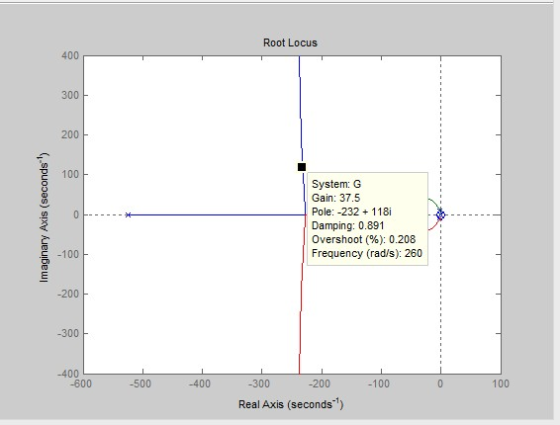
From the rootlocus plot at gain 37.5375 ,there is a dominant pole , since gain of the compensator calculated at dominant pole location.

So the dominant pole location is -232+117i shown below

Root Locus 400 300 200 E 100 System: G Gain: 37.5 Pole: -232 118i Damping: 0.891 Overshoot (%): 0.208 Frequency (rad/s): 260 S -100 -200 -300 -400 100 -600 -500 -300 200 100 -400 Real Axis (seconds)

MATLAB CODE:

clc;
clear all;
close all;
num1=[37.5375 1726.725 1689.1875];%coffients of the numarator polynamial of compensator
den1=[1 525.0325 17.0625];%coffients of the denominator polynamial of compensator
d=tf(num1,den1);% transfer function of compensator
num2=[68];%coffients of the numarator polynamial of plant(system)
den2=[1 4 68];%coffients of the denominator polynamial of plant(system)
gp=tf(num2,den2);% transfer function of plant(system)
G=d*gp;%over all transfer openloop function
figure(1)
%plotting the root locus of the system
rlocus(G)

Solution to (b)

Step Response 1.2 0.8 0.6 0.4 0.2 Time (seconds)

MATLAB CODE:

clc;
clear all;
close all;
num1=[37.5375 1726.725 1689.1875];%coffients of the numarator polynamial of compensator
den1=[1 525.0325 17.0625];%coffients of the denominator polynamial of compensator
d=tf(num1,den1);% transfer function of compensator
num2=[68];%coffients of the numarator polynamial of plant(system)
den2=[1 4 68];%coffients of the denominator polynamial of plant(system)
gp=tf(num2,den2);% transfer function of plant(system)
G=d*gp;%over all transfer openloop function
figure(2)
%plotting step response of the system
step(T)

Solution to(c)

Result are given below

S =
RiseTime: 0.0835 sec
SettlingTime: 3.1334 sec
SettlingMin: 0.6328 sec
SettlingMax: 1.1858 sec
Overshoot: 19.7744
Undershoot: 0
Peak: 1.1858
PeakTime: 0.1697 sec

MATLAB CODE:
clc;
clear all;
close all;
num1=[37.5375 1726.725 1689.1875];%coffients of the numarator polynamial of compensator
den1=[1 525.0325 17.0625];%coffients of the denominator polynamial of compensator
d=tf(num1,den1);% transfer function of compensator
num2=[68];%coffients of the numarator polynamial of plant(system)
den2=[1 4 68];%coffients of the denominator polynamial of plant(system)
gp=tf(num2,den2);% transfer function of plant(system)
G=d*gp;%over all transfer openloop function
T=feedback(G,1);%finding over all closed loop transfer function
%finding the parameters of the system(rise time,settling time,etc)
S=stepinfo(T)

Thankyou