![Question 1-4 is about the following mechanical system: Data: ki-20 [N/m] b-2 [Ns/m] k2# 10 [N/m] m2 At) mi Question 1 X1(s) D](http://img.homeworklib.com/images/5b2d21db-56b1-4a32-a9a1-47ed86dd3c68.png?x-oss-process=image/resize,w_560)
Homework Answers


Add Answer to:
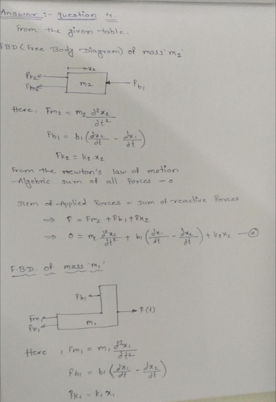
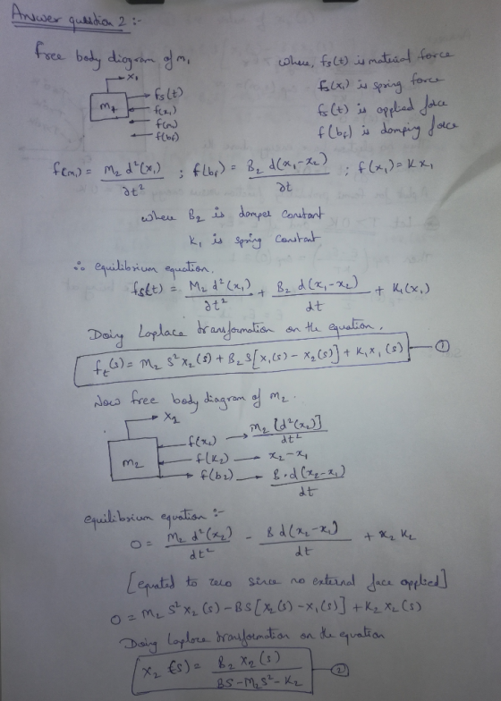
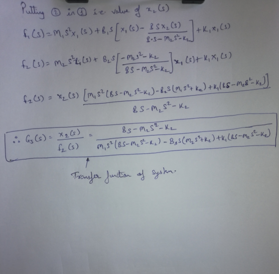
Question 1-4 is about the following mechanical system: Data: ki-20 [N/m] b-2 [Ns/m] k2# 10 [N/m] m2 At) mi Question 1 X...
3. Consider the following mass-spring-damper system. Let m= 1 kg, b = 10 Ns/m, and k...
 3. Consider the following mass-spring-damper system. Let m= 1 kg, b = 10 Ns/m, and k = 20 N/m. b m F k a) Derive the open-loop transfer function X(S) F(s) Plot the step response using matlab. b) Derive the closed-loop transfer function with P-controller with Kp = 300. Plot the step response using matlab. c) Derive the closed-loop transfer function with PD-controller with Ky and Ka = 10. Plot the step response using matlab. d) Derive the closed-loop transfer...
Problem 4. Consider the control system shown below with plant G(s) that has time con- stants...
 Problem 4. Consider the control system shown below with plant G(s) that has time con- stants T1 = 2, T2 = 10, and gain k = 0.1. 4 673 +1679+1) (1.) Sketch the pole-zero plot for G(s). Is one of the poles more dominant? Using MATLAB, simulate the step response of the plant itself, along with G1(s) and G2(s) as defined by Gl(s) = and G2(s) = sti + 1 ST2+1 (2.) Design a proportional gain C(s) = K so...
Mi k2 b yi m2 Figure 5-45 Mechanical system. Assuming that mi 10 kg, m2 5 kg, b 10 N-s/m, k 40 N/...
 mi k2 b yi m2 Figure 5-45 Mechanical system. Assuming that mi 10 kg, m2 5 kg, b 10 N-s/m, k 40 N/m, and k 20 N/m and that input force u is a constant force of 5 N, obtain the response of the sys- tem. Plot the response curves n(t) versus r and y2(t) versus t with MATLAB Problem B-5-23 Consider the system shown in Figure 5-45. The system is at rest for t < 0. The dis placements...
Consider the system. (1) M →1.0) M +0.1 kg, B=0.2 N-s/m Mv(1) + By(t) = 1,01)...
 Consider the system. (1) M →1.0) M +0.1 kg, B=0.2 N-s/m Mv(1) + By(t) = 1,01) Consider a system described by the following differential equation: 0.1"WX2 +0.2v(t) = .0), where y(t) and 4.0) are the output and the input of the system. dt (la) Convert the above differential equation into the form of the typical first-order dynamic system: + ) = ), and explain the physical meaning of the two parameters 7 and v.. (5%) dv(1) (1b) According to the...
1. Consider the system shown. Assume B-3 N-s/m and K-7 N/m. Negligible Mass a) Find the...
 1. Consider the system shown. Assume B-3 N-s/m and K-7 N/m. Negligible Mass a) Find the transfer function, H(s)-X(s)Fa(s) b) Using the transfer function, find the unit step response and the unit impulse response. c) Using the transfer function, find the steady-state response when fa(t) 2 sin (4t) d) Find the free response (zero-input response) assuming x(0) 2 m.
I want the answer for Part B I have the answer for Part A-Q1 I uploaded it 2 H I F ua 212 < > 0.5% on Y; 4Ω Fig...
 I want the answer for Part B I have the answer for Part
A-Q1 I uploaded it
2 H I F ua 212 < > 0.5% on Y; 4Ω Figure 1 PART A: MATHEMATICAL MODEL AND TIME DOMAIN ANALYSIS (5%) 1) For the circuit of Figure 1, determine the transfer function relating the output voltage (s) to the input voltage V(s). Assuming zero initial condition, obtain the output response vo(t) to an input step with 6V amplitude, that is vi(t)6...
I want the answer for Part B I have the answer for Part
A-Q1 I uploaded it
2 H I F ua 212 < > 0.5% on Y; 4Ω Figure 1 PART A: MATHEMATICAL MODEL AND TIME DOMAIN ANALYSIS (5%) 1) For the circuit of Figure 1, determine the transfer function relating the output voltage (s) to the input voltage V(s). Assuming zero initial condition, obtain the output response vo(t) to an input step with 6V amplitude, that is vi(t)6...
A linear time invariant system has an impulse response given by h[n] = 2(-0.5)" u[n] –...
 A linear time invariant system has an impulse response given by h[n] = 2(-0.5)" u[n] – 3(0.5)2º u[n] where u[n] is the unit step function. a) Find the z-domain transfer function H(2). b) Draw pole-zero plot of the system and indicate the region of convergence. c) is the system stable? Explain. d) is the system causal? Explain. e) Find the unit step response s[n] of the system, that is, the response to the unit step input. f) Provide a linear...
Question: given a differential equation: a. initial conditions for the plan and input are zero, ...
 Question:
given a differential equation:
a. initial conditions for the plan and input are zero, derive
plan's transfer function in Laplace transform
b. using inverse Laplace transform, find the solution for the
differential equation for the plan (find function y(t)).
c. derive state-space model of the plan
d. Assume open-loop system with no controller added to the
plant, analyse the steady-state value of the system using final
value theorem and step input
e. Calculate value of the overshoot, rise time...
Question:
given a differential equation:
a. initial conditions for the plan and input are zero, derive
plan's transfer function in Laplace transform
b. using inverse Laplace transform, find the solution for the
differential equation for the plan (find function y(t)).
c. derive state-space model of the plan
d. Assume open-loop system with no controller added to the
plant, analyse the steady-state value of the system using final
value theorem and step input
e. Calculate value of the overshoot, rise time...
are integers and 91 and 92 are 5. Consider the system diagram show in Fig. 2...
 are integers and 91 and 92 are 5. Consider the system diagram show in Fig. 2 for a digital filter. Assume N and M real-valued. (a) Use the diagram to write the difference equation that relates the input to the output. And use the difference equation to write the transfer function for the filter. No Matlab needed. (b) Assume N = 3, M = 5, 91 = 0.5 and 92 = 0.9. Write a Matlab function (call it "ece125filter”) that...
. Question 1 (40 marks) This question asks you to demonstrate your understanding of the following...
 . Question 1 (40 marks) This question asks you to demonstrate your understanding of the following learning objectives LO 1.6 Express the Laplace Transform of common mathematical functions and linear ordinary differential equations using both first principles and mathematical tables. LO 1.7 Construct transfer functions for linear dynamic systems from (i) differential equations and (ii) reduction of block diagrams. LO1.8 Determine the time response of a Linear SISO system to an arbitrary input and having arbitrary initial conditions. LO 1.9...
 3. Consider the following mass-spring-damper system. Let m= 1 kg, b = 10 Ns/m, and k = 20 N/m. b m F k a) Derive the open-loop transfer function X(S) F(s) Plot the step response using matlab. b) Derive the closed-loop transfer function with P-controller with Kp = 300. Plot the step response using matlab. c) Derive the closed-loop transfer function with PD-controller with Ky and Ka = 10. Plot the step response using matlab. d) Derive the closed-loop transfer...
 Problem 4. Consider the control system shown below with plant G(s) that has time con- stants T1 = 2, T2 = 10, and gain k = 0.1. 4 673 +1679+1) (1.) Sketch the pole-zero plot for G(s). Is one of the poles more dominant? Using MATLAB, simulate the step response of the plant itself, along with G1(s) and G2(s) as defined by Gl(s) = and G2(s) = sti + 1 ST2+1 (2.) Design a proportional gain C(s) = K so...
 mi k2 b yi m2 Figure 5-45 Mechanical system. Assuming that mi 10 kg, m2 5 kg, b 10 N-s/m, k 40 N/m, and k 20 N/m and that input force u is a constant force of 5 N, obtain the response of the sys- tem. Plot the response curves n(t) versus r and y2(t) versus t with MATLAB Problem B-5-23 Consider the system shown in Figure 5-45. The system is at rest for t < 0. The dis placements...
 Consider the system. (1) M →1.0) M +0.1 kg, B=0.2 N-s/m Mv(1) + By(t) = 1,01) Consider a system described by the following differential equation: 0.1"WX2 +0.2v(t) = .0), where y(t) and 4.0) are the output and the input of the system. dt (la) Convert the above differential equation into the form of the typical first-order dynamic system: + ) = ), and explain the physical meaning of the two parameters 7 and v.. (5%) dv(1) (1b) According to the...
 1. Consider the system shown. Assume B-3 N-s/m and K-7 N/m. Negligible Mass a) Find the transfer function, H(s)-X(s)Fa(s) b) Using the transfer function, find the unit step response and the unit impulse response. c) Using the transfer function, find the steady-state response when fa(t) 2 sin (4t) d) Find the free response (zero-input response) assuming x(0) 2 m.
 I want the answer for Part B I have the answer for Part
A-Q1 I uploaded it
2 H I F ua 212 < > 0.5% on Y; 4Ω Figure 1 PART A: MATHEMATICAL MODEL AND TIME DOMAIN ANALYSIS (5%) 1) For the circuit of Figure 1, determine the transfer function relating the output voltage (s) to the input voltage V(s). Assuming zero initial condition, obtain the output response vo(t) to an input step with 6V amplitude, that is vi(t)6...
I want the answer for Part B I have the answer for Part
A-Q1 I uploaded it
2 H I F ua 212 < > 0.5% on Y; 4Ω Figure 1 PART A: MATHEMATICAL MODEL AND TIME DOMAIN ANALYSIS (5%) 1) For the circuit of Figure 1, determine the transfer function relating the output voltage (s) to the input voltage V(s). Assuming zero initial condition, obtain the output response vo(t) to an input step with 6V amplitude, that is vi(t)6...
 A linear time invariant system has an impulse response given by h[n] = 2(-0.5)" u[n] – 3(0.5)2º u[n] where u[n] is the unit step function. a) Find the z-domain transfer function H(2). b) Draw pole-zero plot of the system and indicate the region of convergence. c) is the system stable? Explain. d) is the system causal? Explain. e) Find the unit step response s[n] of the system, that is, the response to the unit step input. f) Provide a linear...
 Question:
given a differential equation:
a. initial conditions for the plan and input are zero, derive
plan's transfer function in Laplace transform
b. using inverse Laplace transform, find the solution for the
differential equation for the plan (find function y(t)).
c. derive state-space model of the plan
d. Assume open-loop system with no controller added to the
plant, analyse the steady-state value of the system using final
value theorem and step input
e. Calculate value of the overshoot, rise time...
Question:
given a differential equation:
a. initial conditions for the plan and input are zero, derive
plan's transfer function in Laplace transform
b. using inverse Laplace transform, find the solution for the
differential equation for the plan (find function y(t)).
c. derive state-space model of the plan
d. Assume open-loop system with no controller added to the
plant, analyse the steady-state value of the system using final
value theorem and step input
e. Calculate value of the overshoot, rise time...
 are integers and 91 and 92 are 5. Consider the system diagram show in Fig. 2 for a digital filter. Assume N and M real-valued. (a) Use the diagram to write the difference equation that relates the input to the output. And use the difference equation to write the transfer function for the filter. No Matlab needed. (b) Assume N = 3, M = 5, 91 = 0.5 and 92 = 0.9. Write a Matlab function (call it "ece125filter”) that...
 . Question 1 (40 marks) This question asks you to demonstrate your understanding of the following learning objectives LO 1.6 Express the Laplace Transform of common mathematical functions and linear ordinary differential equations using both first principles and mathematical tables. LO 1.7 Construct transfer functions for linear dynamic systems from (i) differential equations and (ii) reduction of block diagrams. LO1.8 Determine the time response of a Linear SISO system to an arbitrary input and having arbitrary initial conditions. LO 1.9...
Most questions answered within 3 hours.
-
In a survey of 1147 small-business owners, the following
question was posed: Would you recommend working...
asked 21 minutes ago -
The value of the equilibrium constant Kc for the reaction
N2(g)+3H2(g)⇌2NH3(g) changes in the following manner...
asked 28 minutes ago -
There are two flasks on the bench top, one flask contains a 0.50
M NaCl solution...
asked 34 minutes ago -
Which of the following aqueous solutions are good buffer
systems?
.
0.10 M hydrofluoric acid +...
asked 35 minutes ago -
2. An S election is terminated if the S corporation has passive
investment income in excess...
asked 38 minutes ago -
Part of an ANOVA table is shown below.
Source of
Variation
Sum of
Squares
Degrees of...
asked 54 minutes ago -
Business process improvement initiatives often include
introducing new technology to support the new or changed ways...
asked 1 hour ago -
Review your choice of either Agile or the Waterfall models and
for each of the 22...
asked 1 hour ago -
Suppose an x distribution has mean μ = 4.
Consider two corresponding
x
distributions, the first...
asked 1 hour ago -
A study of the effects of exercise used rats bred to have high
or low capacity...
asked 1 hour ago -
Using your data from the experiment, calculate the initial moles
of HCl that you started with....
asked 1 hour ago -
Suppose you want to make 500 mL of a 0.20 M Tris buffer at pH
8.0....
asked 1 hour ago